

ANN and SSO Algorithms for a Newly Developed Flexible Grid Trading Model


Abstract
:1. Introduction
- Provide a new set of grid trading algorithms to improve the shortcomings of premature entry and exit of existing grid trading models in the market.
- Enable the trading algorithm to adapt to change in the external environment as time and market conditions change, and self-adjust the model to reduce investors’ effort in the trading market.
- Reduce the irrational decisions brought about by investors’ subjective trading decisions, through a set of training models with logical rules.
- Balance the relationship between risk and profit, and obtain an excellent reward under a certain reasonable risk.
2. Overview of Grid Trading, SSO, and DL
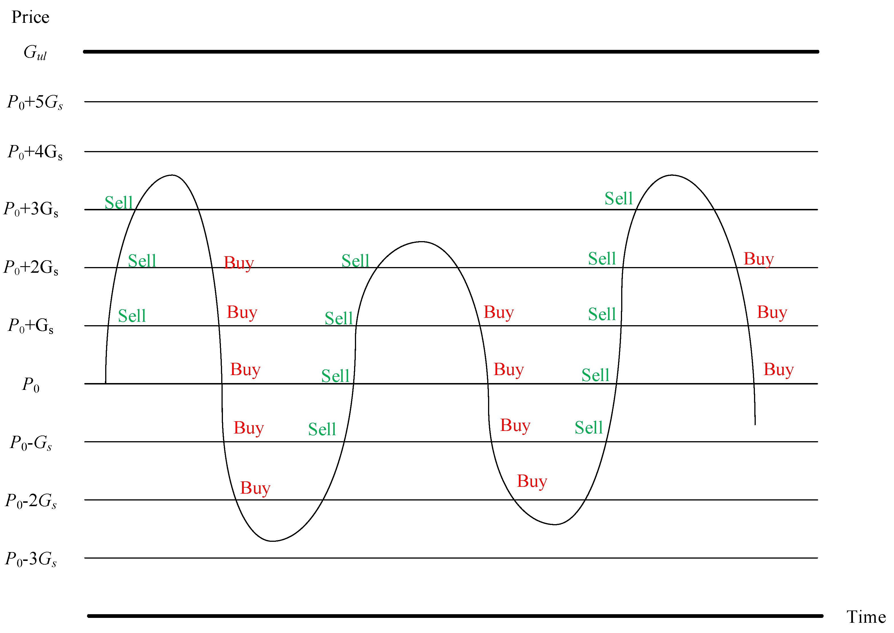
2.1. Grid Trading
2.2. SSO
2.3. DL
2.3.1. ANN
2.3.2. Back-Propagating Method
2.3.3. LSTM
3. Proposed Approach
3.1. Operation Mechanism of Grid Trading
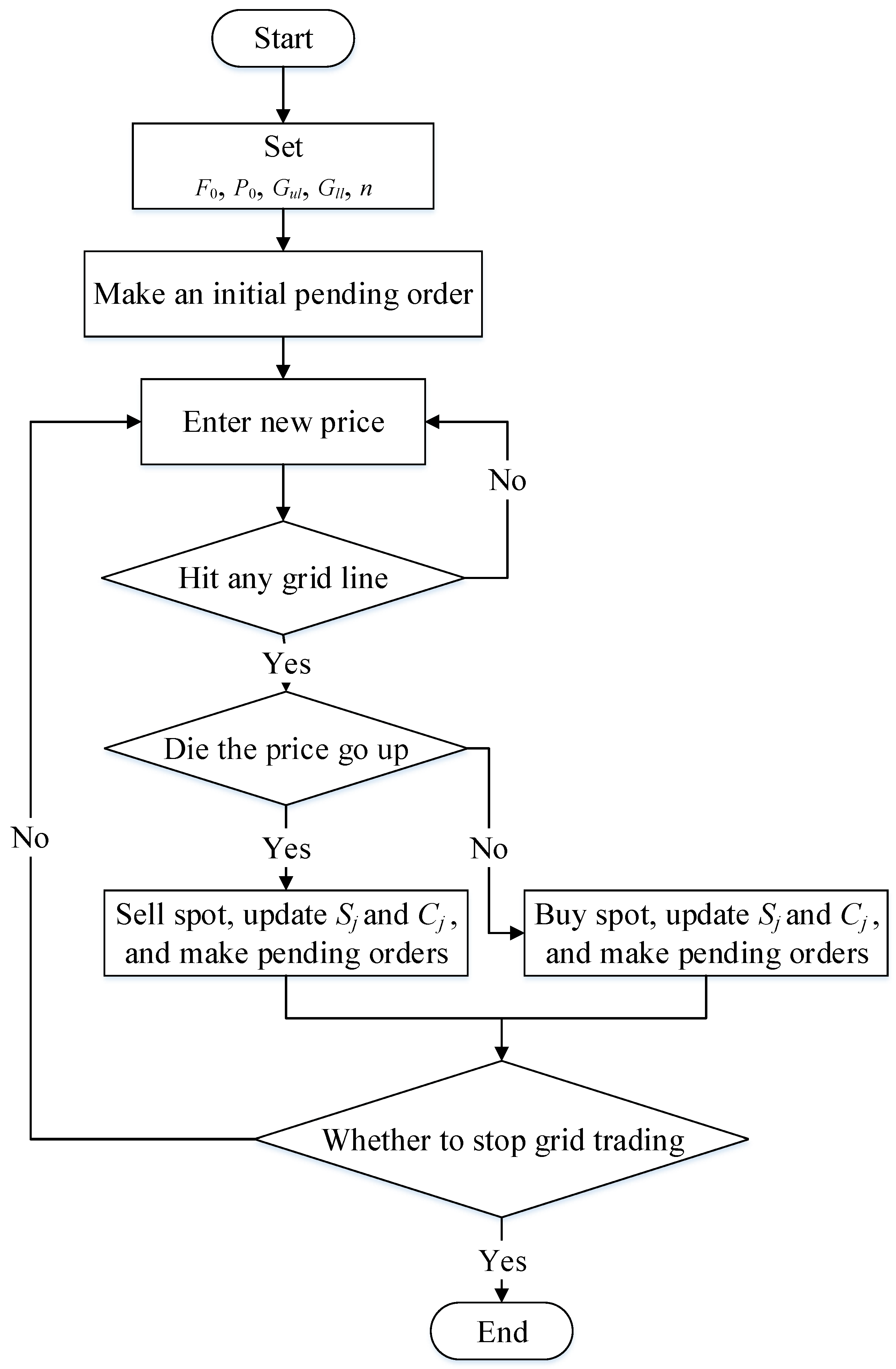
3.1.1. Initial Parameter Setting of Grid Trading
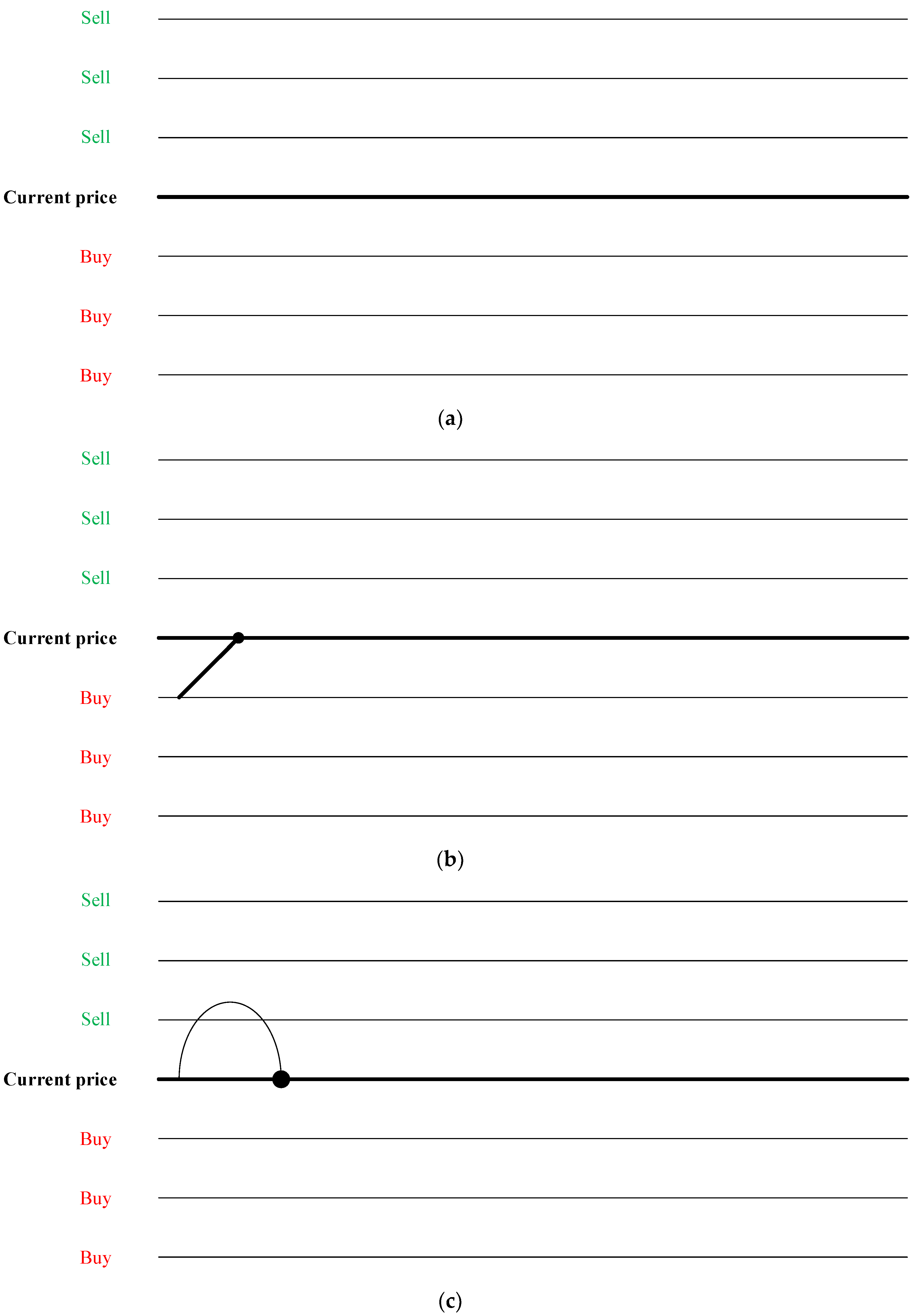
3.1.2. Operation Mechanism of grid Trading
- When the grid is initially running, the current price is used as the benchmark, and the above grid price is placed on a sell order, and the following grid price is placed on a buy order as shown in Figure 3a.
- If the price rises until it hits the first grid line, make a sell action, update the spot volume and funds held, and place a buy order at the original grid position as shown in Figure 3b.
- If the price falls back to the initial grid line, make a buy action, update the spot volume and funds held, and place a sell order at the original grid position as shown in Figure 3c.
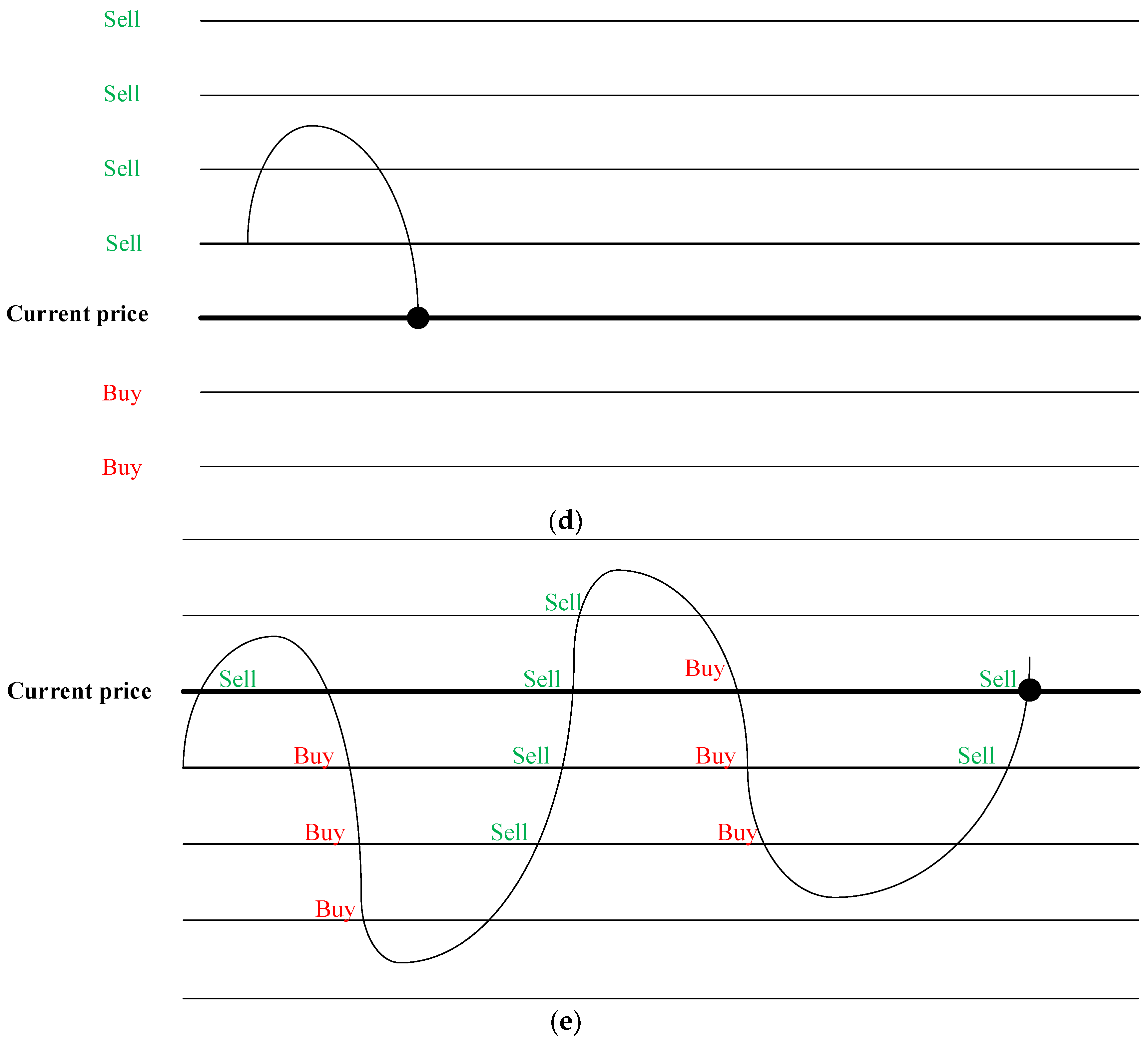
- If the price continues to drop to a grid line, make a buy action, update the spot volume and funds held, and place a sell order at the original grid position as shown in Figure 3d.
- Continue to trade with the above mechanism. Although the price has returned to the original point of grid trading, it has successfully arbitraged seven times, which is equivalent to seven grids of grid spread profits as shown in Figure 3e.
- When the grid trading model is to be closed, there are two ways to end it. One is to directly keep the current spot and funds held, and the other is to sell the spot at the current price and convert it into cash. The former is recommended to be used when the market price is low, and the latter is not recommended. In this study, the grid is closed and settled in the second method.
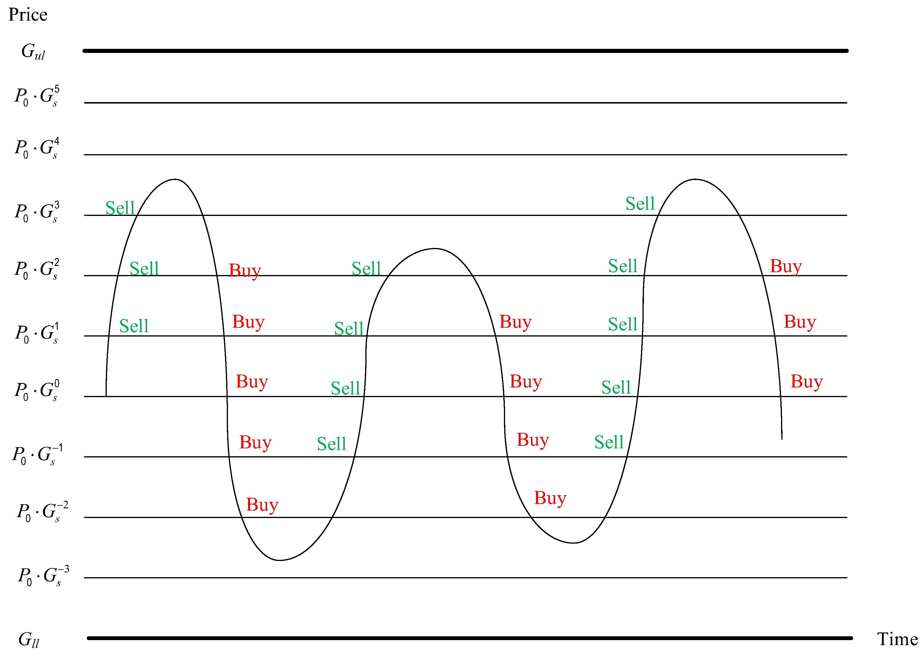
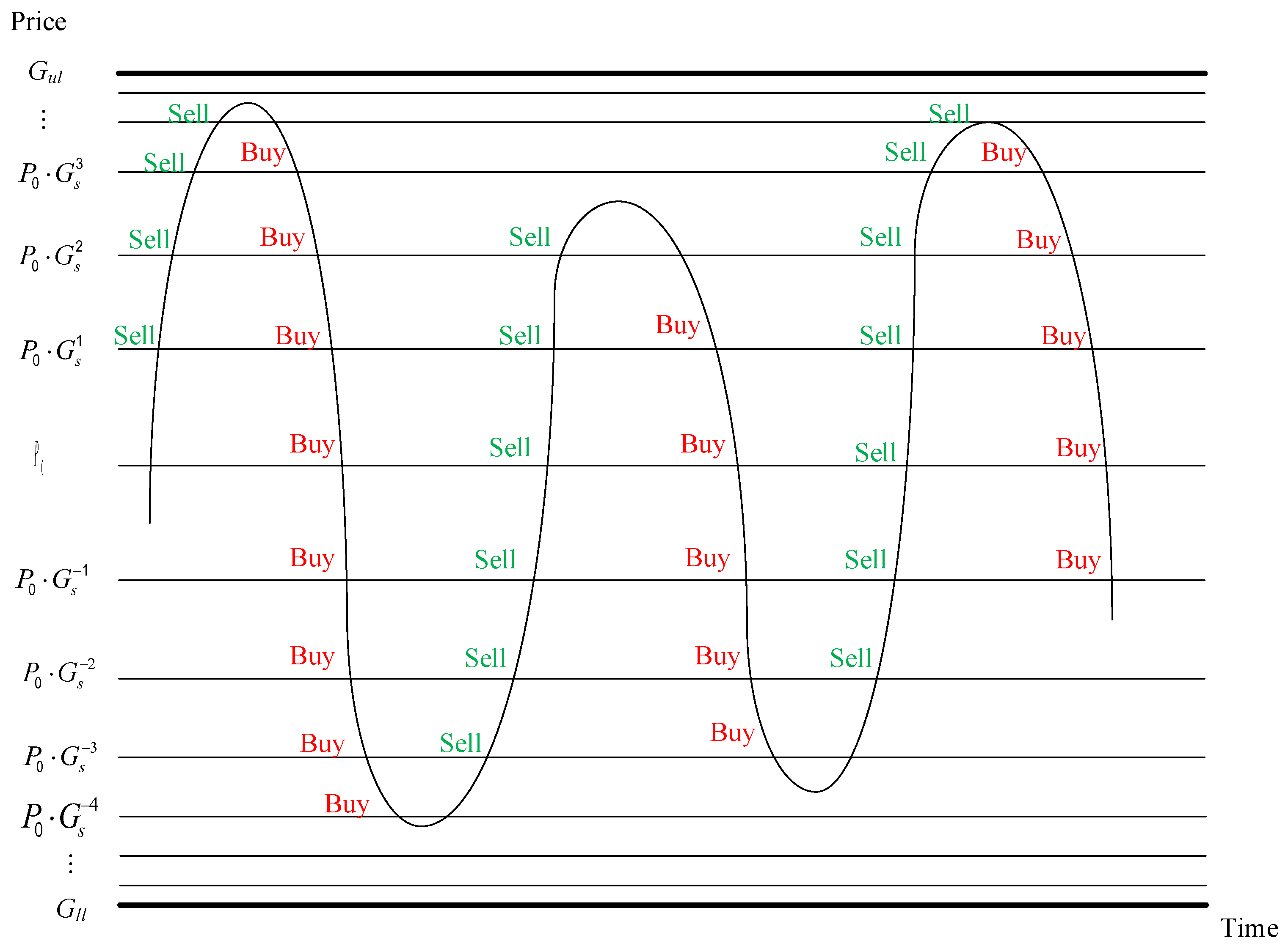
3.2. Concept and Architecture of Flexible Grid
- The number of upper grids nu and the number of lower grids nl in Equation (5) are no longer calculated with Equations (6) and (7) but can be initially set.
- The grid is divided into upper and lower parts with the initial price P0 as the boundary. The upper part and the lower part can set the number of the grids and have their own grid spacing ratio. The ratio of the upper grid spacing is Gsu and the lower grid spacing is Gsl. It should be noted here that Gsu must be a number greater than 0 and less than 1, and Gsl must be a number greater than 1. The feature of this is that the upper grid spacing becomes smaller and smaller as the price is higher, i.e., the trading frequency becomes more and more frequent. Similarly, the lower grid spacing becomes smaller and denser when the price is lower.
3.3. SSO for Optimal Parameters
3.3.1. Objective and Constraint
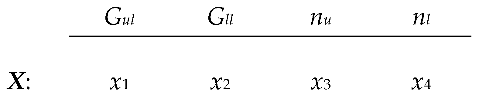
3.3.2. Solution Encoding
3.3.3. Parameter Setting and Scope of Update Mechanism
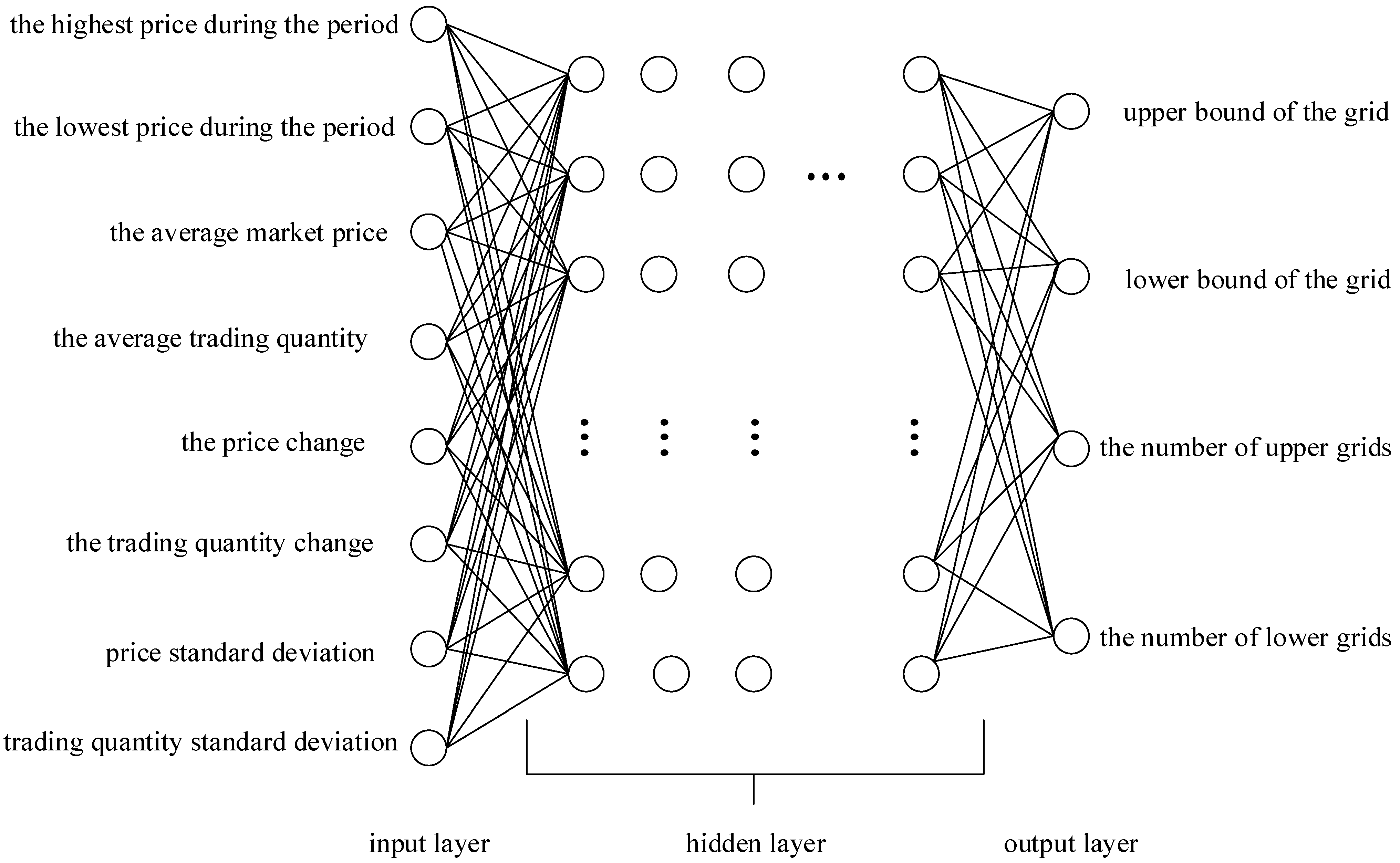
3.4. Training ANN to Automatically Adjust Flexible Grid Parameters
4. Experimental Results
4.1. Verification of Flexible Grid Performance with Fixed Parameters
4.2. SSO Parameter Setting
4.3. Verification of Flexible Grid Performance with Parameters Selected by SSO
4.4. Training ANN to Automatically Adjust Flexible Grid Parameters
5. Conclusions
Author Contributions
Funding
Data Availability Statement
Acknowledgments
Conflicts of Interest
References
- Regulatory Issues Raised by the Impact of Technological Changes on Market Integrity and Efficiency. Consult. Rep, Technical Committee of the International Organization of Securities Commissions. 2011. Available online: https://www.iosco.org/library/pubdocs/pdf/IOSCOPD354.pdf (accessed on 7 October 2022).
- Allen, F.; McAndrews, J.; Strahan, P. E-finance: An introduction. J. Financ. Serv. Res. 2002, 22, 5–27. [Google Scholar] [CrossRef]
- Shahrokhi, M. E-finance: Status, innovations, resources and future challenges. Manag. Financ. 2008, 34, 365–398. [Google Scholar] [CrossRef]
- Turing, A.M. Computing machinery and intelligence. In Parsing the Turing Test; Springer: Dordrecht, The Netherlands, 2009; pp. 23–65. [Google Scholar]
- Hutson, M. How researchers are teaching AI to learn like a child. Science 2018, 10. [Google Scholar] [CrossRef]
- Minsky, M.; Papert, S.A. Perceptrons, Reissue of the 1988 Expanded Edition with a New Foreword by Léon Bottou: An Introduction to Computational Geometry; MIT Press: Cambridge, MA, USA, 2017. [Google Scholar]
- Silver, D.; Huang, A.; Maddison, C.J.; Guez, A.; Sifre, L.; van den Driessche, G.; Schrittwieser, J.; Antonoglou, I.; Panneershelvam, V.; Lanctot, M.; et al. Mastering the game of Go with deep neural networks and tree search. Nature 2016, 529, 484–489. [Google Scholar] [CrossRef] [PubMed]
- Aldridge, I. High-Frequency Trading: A Practical Guide to Algorithmic Strategies and Trading Systems; John Wiley & Sons: New York, NY, USA, 2013; Volume 604. [Google Scholar]
- Lai, Z.-R.; Yang, P.-Y.; Fang, L.; Wu, X. Reweighted price relative tracking system for automatic portfolio optimization. IEEE Trans. Syst. Man Cybern. Syst. 2018, 50, 4349–4361. [Google Scholar] [CrossRef]
- Rundo, F.; Trenta, F.; di Stallo, A.L.; Battiato, S. Grid trading system robot (gtsbot): A novel mathematical algorithm for trading fx market. Appl. Sci. 2019, 9, 1796. [Google Scholar] [CrossRef] [Green Version]
- Wen, Q.; Yang, Z.; Song, Y.; Jia, P. Automatic stock decision support system based on box theory and SVM algorithm. Expert Syst. Appl. 2010, 37, 1015–1022. [Google Scholar] [CrossRef]
- Deng, S.; Sakurai, A. Short-term foreign exchange rate trading based on the support/resistance level of Ichimoku Kinkohyo. In Proceedings of the IEEE International Conference on Information Science, Electronics and Electrical Engineering, Sapporo, Japan, 26–28 April 2014; pp. 337–340. [Google Scholar]
- Ye, A.; Chinthalapati, V.L.R.; Serguieva, A.; Tsang, E. Developing sustainable trading strategies using directional changes with high frequency data. In Proceedings of the IEEE International Conference on Big Data (Big Data), Boston, MA, USA, 11–14 December 2017; pp. 4265–4271. [Google Scholar]
- DuPoly, A. The Expert4x, No stop, Hedged, Grid Trading System and The Hedged, Multi-Currency, Forex Trading System. 2008. Available online: https://c.mql5.com/forextsd/forum/54/grid1.pdf (accessed on 7 October 2022).
- Yeh, W.-C.; Wei, S.-C. Economic-based resource allocation for reliable Grid-computing service based on Grid Bank. Future Gener. Comput. Syst. 2012, 28, 989–1002. [Google Scholar] [CrossRef]
- Wei, S.-C.; Yeh, W.-C. Resource allocation decision model for dependable and cost-effective grid applications based on Grid Bank. Future Gener. Comput. Syst. 2017, 77, 12–28. [Google Scholar] [CrossRef]
- Yeh, W.-C. A two-stage discrete particle swarm optimization for the problem of multiple multi-level redundancy allocation in series systems. Expert Syst. Appl. 2009, 36, 9192–9200. [Google Scholar] [CrossRef]
- Yeh, W.-C. Novel swarm optimization for mining classification rules on thyroid gland data. Inf. Sci. 2012, 197, 65–76. [Google Scholar] [CrossRef]
- Yeh, W.-C.; Chang, W.-W.; Chung, Y.Y. A new hybrid approach for mining breast cancer pattern using discrete particle swarm optimization and statistical method. Expert Syst. Appl. 2009, 36, 8204–8211. [Google Scholar] [CrossRef]
- Yeh, W.-C.; Liu, Z.; Yang, Y.-C.; Tan, S.-Y. Solving dual-channel supply chain pricing strategy problem with multi-level programming based on improved simplified swarm optimization. Technologies 2022, 10, 73. [Google Scholar] [CrossRef]
- Lin, H.C.-S.; Huang, C.-L.; Yeh, W.-C. A novel constraints model of credibility-fuzzy for reliability redundancy allocation problem by simplified swarm optimization. Appl. Sci. 2021, 11, 10765. [Google Scholar] [CrossRef]
- Yeh, W.-C.; Lai, P.-J.; Lee, W.-C.; Chuang, M.-C. Parallel-machine scheduling to minimize makespan with fuzzy processing times and learning effects. Inf. Sci. 2014, 269, 142–158. [Google Scholar] [CrossRef]
- Yeh, W.-C.; Zhu, W.; Tan, S.-Y.; Wang, G.-G.; Yeh, Y.-H. Novel general active reliability redundancy allocation problems and algorithm. Reliab. Eng. Syst. Saf. 2021, 218, 108167. [Google Scholar] [CrossRef]
- Yeh, W.-C.; Tan, S.-Y. Simplified Swarm Optimization for the Heterogeneous Fleet Vehicle Routing Problem with Time-Varying Continuous Speed Function. Electronics 2021, 10, 1775. [Google Scholar] [CrossRef]
- Bae, C.; Yeh, W.C.; Wahid, N.; Chung, Y.Y.; Liu, Y. A new simplified swarm optimization (SSO) using exchange local search scheme. Int. J. Innov. Comput. Inf. Control 2012, 8, 4391–4406. [Google Scholar]
- Yeh, W.-C.; Su, Y.-Z.; Gao, X.-Z.; Hu, C.-F.; Wang, J.; Huang, C.-L. Simplified swarm optimization for bi-objection active reliability redundancy allocation problems. Appl. Soft Comput. 2021, 106, 107321. [Google Scholar] [CrossRef]
- Wang, M.; Yeh, W.-C.; Chu, T.-C.; Zhang, X.; Huang, C.-L.; Yang, J. Solving Multi-Objective Fuzzy Optimization in Wireless Smart Sensor Networks under Uncertainty Using a Hybrid of IFR and SSO Algorithm. Energies 2018, 11, 2385. [Google Scholar] [CrossRef] [Green Version]
- Yeh, W.-C. Simplified swarm optimization in disassembly sequencing problems with learning effects. Comput. Oper. Res. 2012, 39, 2168–2177. [Google Scholar] [CrossRef]
- Yeh, W.-C. A novel boundary swarm optimization method for reliability redundancy allocation problems. Reliab. Eng. Syst. Saf. 2019, 192, 106060. [Google Scholar] [CrossRef]
- Yeh, W.-C. Orthogonal simplified swarm optimization for the series–parallel redundancy allocation problem with a mix of components. Knowl. Based Syst. 2014, 64, 1–12. [Google Scholar] [CrossRef]
- Zhu, W.; Yeh, W.C.; Cao, L.; Zhu, Z.; Chen, D.; Chen, J.; Li, A.; Lin, Y. Faster evolutionary convolutional neural networks based on iSSO for lesion recognition in medical images. Basic Clin. Pharmacol. Toxicol. 2019, 124, 329. [Google Scholar]
- Yeh, W.; Lin, P.; Huang, C. Simplified swarm optimisation for the solar cell models parameter estimation problem. IET Renew. Power Gener. 2017, 11, 1166–1173. [Google Scholar] [CrossRef]
- Lin, P.; Cheng, S.; Yeh, W.; Chen, Z.; Wu, L. Parameters extraction of solar cell models using a modified simplified swarm optimization algorithm. Sol. Energy 2017, 144, 594–603. [Google Scholar] [CrossRef]
- Yeh, W.-C. New Parameter-Free Simplified Swarm Optimization for Artificial Neural Network Training and its Application in the Prediction of Time Series. IEEE Trans. Neural Netw. Learn. Syst. 2013, 24, 661–665. [Google Scholar] [CrossRef] [PubMed]
- Huang, W.; Lai, K.K.; Nakamori, Y.; Wang, S.; Yu, L. Neural networks in finance and economics forecasting. Int. J. Inf. Technol. Decis. Mak. 2007, 6, 113–140. [Google Scholar] [CrossRef]
- Qi, S.; Jin, K.; Li, B.; Qian, Y. The exploration of internet finance by using neural network. J. Comput. Appl. Math. 2020, 369, 112630. [Google Scholar] [CrossRef]
- Siami-Namini, S.; Namin, A.S. Forecasting economics and financial time series: ARIMA vs. LST. arXiv 2018, arXiv:1803.06386. [Google Scholar]
- Cao, J.; Li, Z.; Li, J. Financial time series forecasting model based on CEEMDAN and LST. Phys. A Stat. Mech. Its Appl. 2019, 519, 127–139. [Google Scholar] [CrossRef]
- Jegadeesh, N. Evidence of predictable behavior of security returns. J. Financ. 1990, 45, 881–898. [Google Scholar] [CrossRef]
- Jegadeesh, N. Seasonality in stock price mean reversion: Evidence from the US and the UK. J. Financ. 1991, 46, 1427–1444. [Google Scholar] [CrossRef]
- Li, B.; Zhao, P.; Hoi, S.C.H.; Gopalkrishnan, V. PAMR: Passive aggressive mean reversion strategy for portfolio selection. Mach. Learn. 2012, 87, 221–258. [Google Scholar] [CrossRef]
- Mcculloch, W.S.; Pitts, W.H. A logical calculus of the ideas immanent in nervous activity. Bull. Math. Biophys. 1943, 5, 115–133. [Google Scholar] [CrossRef]
- Rosenblatt, F. The perceptron: A probabilistic model for information storage and organization in the brain. Psychol. Rev. 1958, 65, 386–408. [Google Scholar] [CrossRef] [PubMed] [Green Version]
- Werbos, P. Beyond Regression: New Tools for Prediction and Analysis in the Behavioral Sciences. Ph.D. Thesis, Harvard University, Cambridge, MA, USA, 1974. [Google Scholar]
- Rumelhart, D.E.; Hinton, G.E.; Williams, R.J. Learning representations by back-propagating errors. Nature 1986, 323, 533–536. [Google Scholar] [CrossRef]
- Ruder, S. An overview of gradient descent optimization algorithms. arXiv 2016, arXiv:1609.04747. [Google Scholar]
- Poterba, J.M.; Summers, L.H. Mean reversion in stock prices: Evidence and Implications. J. Financ. Econ. 1988, 22, 27–59. [Google Scholar] [CrossRef]
- Hurst, B.; Ooi, Y.H.; Pedersen, L.H. A century of evidence on trend-following investing. J. Portf. Manag. 2017, 44, 15–29. [Google Scholar] [CrossRef]


| Scope of Use | Parameters | Variable Upper Bound | Variable Lower Bound |
|---|---|---|---|
| Experiment 1 | Grid upper bound Gul | P0 × 130% | P0 × 105% |
| Grid lower bound Gll | P0 × 95% | P0 × 70% | |
| Experiment 2 | Grid upper bound Gul, | P0 × 150% | P0 × 105% |
| Grid lower bound Gll | P0 × 95% | P0 × 50% | |
| In common use | Number of upper grids nu | [P0 × 100/(maximum Px × 1.3)] − 10 | 10 |
| Number of lower grids nl | [P0 × 100/(maximum Px × 1.3)] − 10 | 10 |
| Symbols | Definitions |
|---|---|
| Nvar | The number of variables: the grid upper bound Gul, grid lower bound Gll and total number of grids n in this study. |
| Nsol | Total number of solutions. |
| represents the ith solution in the tth generation, where t = 1, 2,…, Ngen, i = 1, 2, …, Nsol. | |
| pbest and gbest of each variable during the update process. | |
| Cg, Cp, Cw | The three key parameters used to determine the update value in SSO Can be adjusted according to different situations. |
| UB | UB. |
| LB | LB. |
| Grid Type | Flexible Grid | Equal-Distance | Equal-Ratio |
|---|---|---|---|
| S&P 500 (Gul,Gll) = (P0 × 1.3,P0 × 0.7) (Gul,Gll) = (P0 × 1.5,P0 × 0.5) | 31.692% 43.727% | 27.934% 39.556% | 22.234% 30.174% |
| Nasdaq 100 (Gul,Gll) = (P0 × 1.3,P0 × 0.7) (Gul,Gll) = (P0 × 1.5,P0 × 0.5) | 53.795% 71.888% | 49.261% 66.024% | 40.369% 51.180% |
| Dow Jones Industrial Average (Gul,Gll) = (P0 × 1.3,P0 × 0.7) (Gul,Gll) = (P0 × 1.5,P0 × 0.5) | 21.935% 33.541% | 18.332% 29.741% | 13.629% 21.648% |
| Euro Stoxx 50 (Gul,Gll) = (P0 × 1.3,P0 × 0.7) (Gul,Gll) = (P0 × 1.5,P0 × 0.5) | 0.601% 17.499% | −4.122% 12.520% | −7.284% 7.087% |
| Shanghai Composite ((Gul,Gll) = (P0 × 1.3,P0 × 0.7) (Gul,Gll) = (P0 × 1.5,P0 × 0.5) | −33.904% −12.955% | −38.944% −19.936% | −38.534% −18.290% |
| Grid Type | Flexible Grid | Equal-Distance | Equal-Ratio |
|---|---|---|---|
| S&P 500 (Gul,Gll) = (P0 × 1.3,P0 × 0.7) (Gul,Gll) = (P0 × 1.5,P0 × 0.5) | 13,169 14,373 | 12,793 13,956 | 12,223 13,017 |
| Nasdaq 100 (Gul,Gll) = (P0 × 1.3,P0 × 0.7) (Gul,Gll) = (P0 × 1.5,P0 × 0.5) | 15,380 17,189 | 14,926 16,602 | 14,037 15,118 |
| Dow Jones Industrial Average (Gul,Gll) = (P0 × 1.3,P0 × 0.7) (Gul,Gll) = (P0 × 1.5,P0 × 0.5) | 12,194 13,354 | 11,833 12,974 | 11,363 12,165 |
| Euro Stoxx 50 (Gul,Gll) = (P0 × 1.3,P0 × 0.7) (Gul,Gll) = (P0 × 1.5,P0 × 0.5) | 10,060 11,750 | 9588 11,252 | 9272 10,709 |
| Shanghai Composite (Gul,Gll) = (P0 × 1.3,P0 × 0.7) (Gul,Gll) = (P0 × 1.5,P0 × 0.5) | 6610 8705 | 6106 8006 | 6147 8171 |
| Grid Type | Flexible Grid | Equal-Distance | Equal-Ratio |
|---|---|---|---|
| S&P 500 (Gul,Gll) = (P0 × 1.3,P0 × 0.7) (Gul,Gll) = (P0 × 1.5,P0 × 0.5) | 0.118 0.160 | 0.103 0.145 | 0.092 0.137 |
| Nasdaq 100 (Gul,Gll) = (P0 × 1.3,P0 × 0.7) (Gul,Gll) = (P0 × 1.5,P0 × 0.5) | 0.187 0.234 | 0.172 0.219 | 0.161 0.215 |
| Dow Jones Industrial Average (Gul,Gll) = (P0 × 1.3,P0 × 0.7) (Gul,Gll) = (P0 × 1.5,P0 × 0.5) | 0.079 0.119 | 0.065 0.105 | 0.054 0.095 |
| Euro Stoxx 50 (Gul,Gll) = (P0 × 1.3,P0 × 0.7) (Gul,Gll) = (P0 × 1.5,P0 × 0.5) | 0.002 0.046 | −0.011 0.033 | −0.021 0.023 |
| Shanghai Composite (Gul,Gll) = (P0 × 1.3,P0 × 0.7) (Gul,Gll) = (P0 × 1.5,P0 × 0.5) | −0.082 −0.030 | −0.095 −0.047 | −0.106 −0.053 |
| (Cg,Cp,Cw) | Maximum Scale Solution | ROI (Max) | ROI (Min) |
|---|---|---|---|
| (0.7,0.8,0.9) | gbest | 69.74% | 66.83% |
| (0.1,0.8,0.9) | pbest | 69.62% | 67.18% |
| (0.1,0.2,0.9) | 69.69% | 66.01% | |
| (0.1,0.2,0.3) | proposed solution | 69.41% | 66.69% |
| (Cg,Cp,Cw) | Maximum Scale Solution | ROI (Max) | ROI (Min) |
|---|---|---|---|
| (0.5,0.8,0.9) | pbest | 69.77% | 66.22% |
| (0.5,0.6,0.9) | 69.77% | 66.91% | |
| (0.5,0.6,0.7) | proposed solution | 69.86% | 67.83% |
| (Cg,Cp,Cw) | Maximum Scale Solution | ROI (Max) | ROI (Min) |
|---|---|---|---|
| (0.3,0.6,0.7) | pbest | 69.85% | 67.99% |
| (0.3,0.4,0.7) | 69.90% | 67.81% |
| Grid Type | Flexible Grid | Equal-Distance | Equal-Ratio |
|---|---|---|---|
| S&P 500 (Gul,Gll) = (P0 × 1.3,P0 × 0.7) (Gul,Gll) = (P0 × 1.5,P0 × 0.5) | 82.859% 90.269% | 66.384% 77.198% | 58.394% 60.774% |
| Nasdaq 100 (Gul,Gll) = (P0 × 1.3,P0 × 0.7) (Gul,Gll) = (P0 × 1.5,P0 × 0.5) | 111.649% 127.268% | 66.384% 110.179% | 82.662% 86.208% |
| Dow Jones Industrial Average (Gul,Gll) = (P0 × 1.3,P0 × 0.7) (Gul,Gll) = (P0 × 1.5,P0 × 0.5) | 74.509% 80.559% | 60.591% 70.063% | 51.893% 54.760% |
| Euro Stoxx 50 (Gul,Gll) = (P0 × 1.3,P0 × 0.7) (Gul,Gll) = (P0 × 1.5,P0 × 0.5) | 77.220% 88.844% | 56.650% 72.293% | 48.365% 55.856% |
| Shanghai Composite (Gul,Gll) = (P0 × 1.3,P0 × 0.7) (Gul,Gll) = (P0 × 1.5,P0 × 0.5) | 58.389% 80.954% | 39.178% 58.934% | 33.363% 43.639% |
| Grid Type | Flexible Grid | Equal-Distance | Equal-Ratio |
|---|---|---|---|
| S&P 500 (Gul,Gll) = (P0 × 1.3,P0 × 0.7) (Gul,Gll) = (P0 × 1.5,P0 × 0.5) | 18,286 19,027 | 16,638 17,720 | 15,839 16,077 |
| Nasdaq 100 (Gul,Gll) = (P0 × 1.3,P0 × 0.7) (Gul,Gll) = (P0 × 1.5,P0 × 0.5) | 21,165 22,727 | 16,638 21,018 | 18,266 18,621 |
| Dow Jones Industrial Average (Gul,Gll) = (P0 × 1.3,P0 × 0.7) (Gul,Gll) = (P0 × 1.5,P0 × 0.5) | 17,451 18,056 | 16,059 17,006 | 15,189 15,476 |
| Euro Stoxx 50 (Gul,Gll) = (P0 × 1.3,P0 × 0.7) (Gul,Gll) = (P0 × 1.5,P0 × 0.5) | 17,722 18,884 | 15,665 17,229 | 14,837 15,586 |
| Shanghai Composite (Gul,Gll) = (P0 × 1.3,P0 × 0.7) (Gul,Gll) = (P0 × 1.5,P0 × 0.5) | 15,839 18,095 | 13,918 15,893 | 13,336 14,364 |
| Grid Type | Flexible Grid | Equal-Distance | EQUAL-RATIO |
|---|---|---|---|
| S&P 500 (Gul,Gll) = (P0 × 1.3,P0 × 0.7) (Gul,Gll) = (P0 × 1.5,P0 × 0.5) | 0.439 0.442 | 0.350 0.391 | 0.351 0.388 |
| Nasdaq 100 (Gul,Gll) = (P0 × 1.3,P0 × 0.7) (Gul,Gll) = (P0 × 1.5,P0 × 0.5) | 0.498 0.524 | 0.350 0.464 | 0.437 0.462 |
| Dow Jones Industrial Average (Gul,Gll) = (P0 × 1.3,P0 × 0.7) (Gul,Gll) = (P0 × 1.5,P0 × 0.5) | 0.377 0.412 | 0.310 0.344 | 0.301 0.341 |
| Euro Stoxx 50 (Gul,Gll) = (P0 × 1.3,P0 × 0.7) (Gul,Gll) = (P0 × 1.5,P0 × 0.5) | 0.300 0.331 | 0.219 0.265 | 0.211 0.257 |
| Shanghai Composite (Gul,Gll) = (P0 × 1.3,P0 × 0.7) (Gul,Gll) = (P0 × 1.5,P0 × 0.5) | 0.189 0.220 | 0.134 0.179 | 0.131 0.172 |
| Item | Value Set |
|---|---|
| Number of input variables | 8 |
| Number of hidden layers | 3 |
| Number of output variables | 4 |
| Number of hidden layer nodes | 500 |
| Optimizer | adam |
| Excitation function | sigmoid |
| Loss function | mean squared error |
| Number of generations | 300 |
| Batch size | 40 |
| Item | Value Set |
|---|---|
| Number of input variables | 8 |
| Number of hidden layers | 3 |
| Number of output variables | 4 |
| Number of hidden layer nodes | 256, 128, 64 |
| Optimizer | adam |
| Excitation function | relu |
| Loss function | mean squared error |
| Number of generations | 300 |
| Batch size | 32 |
| Neural Network Type | FNN | LSTM |
|---|---|---|
| S&P 500 Upper bound of the grid Gul Lower bound of the grid Gll Number of upper grids nu Number of lower grids nl | 129,510 59,787 207 308 | 186,366 108,622 252 442 |
| Nasdaq 100 Upper bound of the grid Gul Lower bound of the grid Gll Number of upper grids nu Number of lower grids nl | 4,725,772 1,681,699 133 246 | 518,181 1,162,381 296 568 |
| Dow Jones Industrial Average Upper bound of the grid Gul Lower bound of the grid Gll Number of upper grids nu Number of lower grids nl | 6,016,533 2,011,354 164 319 | 24,446,812 19,594,848 237 402 |
| Euro Stoxx 50 Upper bound of the grid Gul Lower bound of the grid Gll Number of upper grids nu Number of lower grids nl | 105,024 33,988 132 199 | 334,456 106,422 202 290 |
| Shanghai Composite Upper bound of the grid Gul Lower bound of the grid Gll Number of upper grids nu Number of lower grids nl | 65,199 33,604 85 214 | 92,869 26,189 280 459 |
| Neural Network Type | FNN | LSTM |
|---|---|---|
| S&P 500 Upper bound of the grid Gul Uower bound of the grid Gll Number of upper grids nu Number of lower grids nl | 97.410% 99.586% 94.972% 99.392% | 90.490% 90.490% 97.240% 99.469% 94.892% |
| Nasdaq 100 Upper bound of the grid Gul Lower bound of the grid Gll Number of upper grids nu Number of lower grids nl | 96.415% 97.088% 94.942% 94.737% | 98.075% 99.915% 99.635% 98.019% |
| Dow Jones Industrial Average Upper bound of the grid Gul Lower bound of the grid Gll Number of upper grids nu Number of lower grids nl | 97.704% 99.771% 99.855% 99.559% | 95.970% 93.429% 93.685% 91.285% |
| Euro Stoxx 50 Upper bound of the grid Gul Lower bound of the grid Gll Number of upper grids nu Number of lower grids nl | 96.183% 99.324% 99.297% 98.405% | 94.392% 98.063% 96.858% 99.760% |
| Shanghai Composite Upper bound of the grid Gul Lower bound of the grid Gll Number of upper grids nu Number of lower grids nl | 97.157% 96.749% 93.165% 99.661% | 96.577% 95.545% 93.881% 99.003% |
| S&P | Nasdaq | DJI | Euro Stoxx | Shanghai | |
|---|---|---|---|---|---|
| B&S | 14.392% | 1.519% | 9.880% | 28.340% | −15.581% |
| S&B | −14.392% | −1.519% | −9.880% | −28.340% | 15.581% |
| GTSbot | 6.408% | 4.680% | 6.594% | 1.191% | −0.466% |
| IWOC | 24.111% | 23.171% | 7.143% | 32.087% | −18.758% |
| FG-FNN | 11.520% | 11.733% | 8.849% | 12.977% | −3.125% |
| FG-LSTM | 4.639% | 1.823% | 2.940% | 7.734% | −9.283% |
| Equal-distance | 5.194% | −2.972% | 3.480% | 10.748% | −4.495% |
| Equal-ratio | 4.536% | −3.625% | 3.276% | 10.764% | −4.892% |
| Flexible | 5.589% | −1.895% | 4.270% | 11.477% | −4.309% |
| S&P | Nasdaq | DJI | Euro Stoxx | Shanghai | |
|---|---|---|---|---|---|
| B&S | 7.960% | 12.570% | 7.290% | 4.029% | 8.529% |
| S&B | 7.491% | 10.370% | 6.580% | 7.313% | 3.103% |
| GTSbot | 0.524% | 5.335% | 1.000% | 0.510% | 1.126% |
| IWOC | 10.345% | 12.421% | 8.606% | 5.467% | 7.640% |
| FG-FNN | 6.455% | 5.596% | 7.491% | 2.034% | 4.105% |
| FG-LSTM | 1.580% | 49.031% | 4.809% | 2.966% | 3.551% |
| Equal-distance | 5.252% | 8.594% | 4.078% | 1.513% | 4.074% |
| Equal-ratio | 5.243% | 10.096% | 4.057% | 1.529% | 4.059% |
| Flexible | 4.737% | 8.780% | 4.163% | 4.144% | 4.208% |
| S&P | Nasdaq | DJI | Euro Stoxx | Shanghai | |
|---|---|---|---|---|---|
| B&S | 0.06126 | 0.07671 | 0.03568 | 0.06221 | 0.01840 |
| S&B | 0.06126 | 0.07671 | 0.03568 | 0.06221 | 0.01840 |
| GTSbot | 0.01710 | 0.03589 | 0.01795 | 0.00267 | 0.00190 |
| IWOC | 0.07689 | 0.08398 | 0.04564 | 0.07337 | 0.03568 |
| FG-FNN | 0.01687 | 0.02076 | 0.02149 | 0.01730 | 0.01414 |
| FG-LSTM | 0.01672 | 0.01637 | 0.02203 | 0.01679 | 0.02030 |
| Equal-distance | 0.02450 | 0.03579 | 0.02129 | 0.01786 | 0.01590 |
| Equal-ratio | 0.02473 | 0.03629 | 0.02155 | 0.01828 | 0.01629 |
| Flexible | 0.02503 | 0.03665 | 0.02162 | 0.01862 | 0.01624 |
| S&P | Nasdaq | DJI | Euro Stoxx | Shanghai | |
|---|---|---|---|---|---|
| B&S | 2.349 | 0.198 | 2.769 | 4.556 | −8.466 |
| S&B | −2.349 | −0.198 | −2.769 | −4.556 | 8.466 |
| GTSbot | 3.748 | 1.304 | 3.673 | 4.466 | −2.446 |
| IWOC | 3.136 | 2.759 | 1.565 | 4.373 | −5.258 |
| FG-FNN | 6.828 | 5.651 | 4.119 | 7.499 | −2.210 |
| FG-LSTM | 2.774 | 1.114 | 1.335 | 4.606 | −4.573 |
| Equal-distance | 2.120 | −0.830 | 1.634 | 6.017 | −2.827 |
| Equal-ratio | 1.834 | −0.999 | 1.520 | 5.887 | −3.004 |
| Flexible | 2.233 | −0.517 | 1.975 | 6.165 | −2.653 |
Publisher’s Note: MDPI stays neutral with regard to jurisdictional claims in published maps and institutional affiliations. |
© 2022 by the authors. Licensee MDPI, Basel, Switzerland. This article is an open access article distributed under the terms and conditions of the Creative Commons Attribution (CC BY) license (https://creativecommons.org/licenses/by/4.0/).
Share and Cite
Yeh, W.-C.; Hsieh, Y.-H.; Hsu, K.-Y.; Huang, C.-L. ANN and SSO Algorithms for a Newly Developed Flexible Grid Trading Model. Electronics 2022, 11, 3259. https://doi.org/10.3390/electronics11193259
Yeh W-C, Hsieh Y-H, Hsu K-Y, Huang C-L. ANN and SSO Algorithms for a Newly Developed Flexible Grid Trading Model. Electronics. 2022; 11(19):3259. https://doi.org/10.3390/electronics11193259
Chicago/Turabian StyleYeh, Wei-Chang, Yu-Hsin Hsieh, Kai-Yi Hsu, and Chia-Ling Huang. 2022. "ANN and SSO Algorithms for a Newly Developed Flexible Grid Trading Model" Electronics 11, no. 19: 3259. https://doi.org/10.3390/electronics11193259
APA StyleYeh, W.-C., Hsieh, Y.-H., Hsu, K.-Y., & Huang, C.-L. (2022). ANN and SSO Algorithms for a Newly Developed Flexible Grid Trading Model. Electronics, 11(19), 3259. https://doi.org/10.3390/electronics11193259