Fault Diagnosis of Vibration Sensors Based on Triage Loss Function-Improved XGBoost

Abstract

Vibration sensors are prone to bias, drift, and other failures. To avoid misjudgments in state monitoring systems and potential safety accidents caused by vibration sensor failures, it is significant to diagnose the faults of vibration sensors. Existing methods for vibration sensor fault diagnosis are primarily based on Deep Learning, but Extreme Gradient Boosting stands out due to its excellent interpretability, and compared to other ensemble learning algorithms, it boasts superior accuracy and efficiency. Therefore, a vibration sensor fault diagnosis method based on Extreme Gradient Boosting is proposed to diagnose seven common types of faults in vibration sensors. To prevent the model from being overwhelmed by simple negative cases during training, a new loss function named Triage Loss is designed to improve the classifier’s performance. The vibration sensor fault diagnosis has confirmed the efficacy and practicality of the suggested approach. The experimental results indicate that the training of the model done using Triage Loss outperforms the training model done using the default loss function, with a maximum improvement of 5.4% accuracy, 5.45% in the F1-score, and 9.87% in the mean Average Precision under different fault rates.

1. Introduction

Reliability and safety of equipment in industrial production processes are critical concerns, and equipment health monitoring has received widespread attention [1,2]. Sensor measurements provide real-time information about the operating status of equipment. However, when sensors malfunction or provide inaccurate readings, it can result in misjudgments in control systems. In industrial production, the lifespan of equipment is often much longer than that of sensors, leading to situations where sensors may fail before the equipment. Therefore, the vibration sensor fault diagnosis (VSFD) is particularly important.

The methods for sensor fault diagnosis mainly include hardware redundancy, analytic redundancy, model-based methods, and Machine Learning (ML)-based methods. In hardware redundancy, two or more sensors are used to measure the same physical quantity, and Barberree [3] designed a self-validating temperature sensor based on this principle. Analytic redundancy utilizes the correlation between sensors to detect the fault, and Wang [4] proposed a fault detection method for flow sensors and temperature sensors based on this approach. In model-based methods, by establishing a system output model, one can calculate the discrepancy between the outputs of the model and the system and then judge whether there is a fault based on the set threshold. Willsky [5] initially proposed this method. Ferdowsi [6] proposes a new model-based method to diagnose nonlinear systems’ faults, including sudden and early faults and the duration of fault occurrence. Ng [7] used a Bayesian approach combined with the physical relationship between water flow and temperature in a pipeline system to develop a model for detecting deviations in sensors of chilled water plant. Yu [8] proposed an improved model based on voltage and current for current sensor diagnosis. Hardware redundancy may incur high costs and complexity in industrial equipment with limited redundancy. Analytic redundancy does not require additional hardware, but is susceptible to noise and relies on empirical analysis, which may compromise reliability. Model-based methods depend on accurate models, which are challenging to establish in practice, especially for systems with nonlinear dynamics and complex sensor behaviors.

Over the past few years, due to the emergence of ML, machine learning has shown a strong performance in fault diagnosis, and the application of early fault diagnosis in equipment has become widespread. Jana [9] used convolutional neural networks to achieve sensor fault diagnosis. Sun [10] collected experimental data on gas turbines under different working conditions, and a database of five typical faults was established. An ML-based method was used to achieve higher diagnostic accuracy for gas turbine sensors. Gao [11] mainly aimed at the drift fault of the chiller sensor. The residual generator generates the residual vector, and the accumulated residual improves the fault detection ability of the model. Ai [12] used a Temporal Convolutional Network for diagnosing Hypersonic Air Vehicle sensors. Xiao [13] used regularized extreme machine learning to detect sensors at different circuit positions. Niu [14] used principal component analysis and improved the Petri net to analyze the speed data of high-speed trains, and the intermittent fault or time-varying fault of the speed sensor was diagnosed. Elnour [15] used auto-associative neural networks to diagnose HVAC system sensors. Although deep neural networks show a strong performance, they have long been criticized for their poor interpretability. In addition, there are some methods for the fault diagnosis of sensors using prediction methods, for example [16,17], Facebook’s Prophet, the Auto-regressive Integrated Moving Average, and other models, which are used to predict the output of sensors. When the actual output exceeds the predicted upper and lower bounds, it is judged as an anomaly, but such methods usually cannot detect the sensor fault type.

Extreme Gradient Boosting (XGBoost) [18], based on decision trees, has been recognized for its excellent interpretability and advantages of requiring less training data and a shorter training time. XGBoost has demonstrated high accuracy and efficiency compared to other ensemble learning algorithms [19,20,21,22], making it widely applied in classification and regression tasks. This paper proposed a VSFD method based on XGBoost to address the seven common fault recognition issues related to vibration sensors. By inputting historical data into XGBoost for training, a classifier is obtained for diagnosing common faults in vibration sensors. Historical data for vibration sensor faults are often imbalanced; the class imbalance in the data can result in the model’s loss being heavily dominated by the majority class during the training process, leading to poor accuracy. Therefore, the Triage loss (TL) was designed for training XGBoost, aiming to address this issue. By introducing a dynamic scaling factor, the model can dynamically scale loss based on the predicted difficulty of the sample. Ultimately, this results in the better classification accuracy and performance of the classifier in classifying faults in vibration sensors.

• This paper proposed a VSFD method based on XGBoost, which can identify seven common faults in vibration sensors. The method exhibits high accuracy.
• In order to prevent the model from being overwhelmed by simple negative samples in the training process, a new loss function TL is designed to train XGBoost, thereby improving the classification performance of the model.
• Finally, the performance of the classification model trained by the default loss function (softmax), focal loss function (FL), and TL is evaluated by experiments on both public and experimental datasets. The results show that the TL-trained model has a higher classification accuracy and better comprehensive performance.

The rest of the paper is as follows: In Section 2, the common types of faults in vibration sensors were introduced. Section 3 presents the proposed method in detail. In Section 4, the experimental validation of the method is conducted. Finally, in Section 5, the paper is summarized.

2. Basic Theory of Typical Faults of Sensors

Deviations between the sensor outputs and expected behavior are considered faults. This paper finds seven common faults in vibration sensors, including bias fault, drift fault, spike fault, data-loss fault, stuck fault, erratic fault, and random faults, to identify the early stages of sensor faults, as shown in Figure 1. $s\left(t\right)=h\left(t\right)+\eta$ is defined as the expected output of the sensor in the absence of faults, where $h\left(t\right)+\eta$, representing the data collected at time t, and $\eta ~N(0,{\delta }_{\eta }^2)$ is noise. The definitions of different types of faults are as follows:

• Bias fault

If the expected output is increased by a constant value, it may result in a deviation from the usual value, which could be due to the poor calibration of the sensor unit or a short circuit. This fault is represented by Equation (1):

$$s\left(t\right)=h\left(t\right)+\eta +v,v=constant$$

(1)

• Drift fault

When the expected output increases linearly with time, it is called a drift fault. Possible causes of this type of fault include material corrosion over time in the sensor or physical damage caused under extreme conditions. This fault is represented by Equation (2):

$$s\left(t\right)=h\left(t\right)+\eta +b\left(t\right),b\left(t\right)=b(t-1)+v$$

(2)

where $b\left(t\right)$ is the bias that varies over time added to the output at time t, which grows linearly with time.

• Spike fault

When the sensor’s output exhibits sharp spikes at regular intervals, it is referred to as a spike fault. This is caused by abnormal vibrations from other system components, affecting the sensor’s output. This fault is represented by Equation (3):

$$s\left(t\right)=\left\{h\right(t)+\eta +v(t);\forall t=v\times \tau ,h(t)+\eta ; otherwise,v=\{\mathrm{1,2},\dots \}, \tau \ge 2$$

(3)

where $\tau$ represents the time interval at which the spikes occur.

• Erratic/precision degradation fault

When a noise with zero mean and high variance is added to the sensor output, resulting in significantly higher friction than the normal state, it is called an accuracy degradation fault. This could be due to sparse connections in the circuit, high-frequency noise in the system, or physical damage. This fault is represented by Equation (4):

$$s\left(t\right)=h\left(t\right)+\eta +v,v~N(0,{\delta }_v^2),{\delta }_v^2\gg {\delta }_n^2$$

(4)

• Stuck fault

When the output of a sensor is stuck at a fixed value temporarily or permanently, it is referred to as a stuck fault. Short circuits, open circuits, or sensor material damage in the circuitry may cause this. This fault is represented by Equation (5):

$$s\left(t\right)=v$$

(5)

• Data-loss fault

A data-loss fault is when the sensor output detects missing values in the time series. This is primarily caused by hardware damage or improper calibration.

• Random faults

Random faults are characterized by the occurrence of multiple positive or negative disturbances in the output of the sensor, which happen very rapidly and may be attributed to the random occurrence of the faults described earlier.

3. Proposed Method

The proposed method is a VSFD method based on XGBoost. In the training process of the XGBoost model, the loss is often occupied by simple negative classes, which leads to a decrease in diagnostic accuracy. Therefore, TL was designed for training XGBoost, aiming to address this issue.

3.1. XGBoost

XGBoost is an additive model based on the improvement of Gradient Boosting Decision Trees (GBDT). In comparison to the GBDT that utilizes a first-order Taylor expansion for the objective function, XGBoost employs a second-order Taylor, incorporating both first-order and second-order derivative information. This feature makes the XGBoost more accurate.

3.2. Triage Loss

We are optimizing the objective function by adjusting model parameters to achieve better performance on the test set to achieve the purpose of learning. The Loss function is utilized to calculate the error between the real value and the predicted value, and the regularization term used to prevent the model from overfitting constitutes the objective function of XGBoost.

For a dataset $\mathcal{D}=\left\{\right({\mathrm{x}}_i,y_i\left)\right\}\left(\right|\mathcal{D}|=n,{\mathrm{x}}_i\in {\mathbb{R}}^m,y_i\in \mathbb{R})$ with n examples and m features, the K additive functions are used to predict the outputs.

$${\widehat{y}}_i=\mathrm{\varnothing }\left({\mathrm{x}}_i\right)={\sum }_{K=1}^K{f}_k\left({\mathrm{x}}_i\right),\hspace{1em}\hspace{1em}{f}_k\in \mathcal{F}$$

(6)

where $\mathcal{F}=\left\{f\right(\mathrm{x})={\omega }_{q\left(\mathrm{x}\right)}\}:(q:{\mathbb{R}}^m\to T, \omega \in {\mathbb{R}}^T)$ is the space of regression trees, where $q$ represents the structure of each regression tree, and T is the number of leaf nodes. $f_k$ depends on q and weight w, and different q and weight w will result in different $f_k$. The objective function of XGBoost is defined as:

$${\mathcal{L}}^{\left(t\right)}={\sum }_{i=1}^{n}l(y_i,{\widehat{y}}_i^{(t-1)}+f_t({\mathrm{x}}_i\left)\right)+\mathsf{\Omega }\left(f_t\right)$$

(7)

where $\mathsf{\Omega }\left(f_t\right)=\gamma T+\lambda {‖\omega ‖}^2/2$, $l$ is a second-order differentiable convex loss function, used to measure the difference between predicted values ${\widehat{y}}_i$ and true values $y_i$. This makes the objective function non-continuous and difficult to optimize. Hence, the objective function can be approximated through the second-order Taylor expansion, making it easier to optimize.

$${\mathcal{L}}^{\left(t\right)}\simeq {\sum }_{i=1}^n\left[l\right(y_i,{\widehat{y}}^{(t-1)})+g_i{f}_t({\mathrm{x}}_i)+h_i{f}_t^2({\mathrm{x}}_i)/2)]+\mathsf{\Omega }(f_t)$$

(8)

where $g_i={\partial }_{{\widehat{y}}^{(t-1)}}l(y_i, {\widehat{y}}^{(t-1)})$ and $h_i={\partial }_{{\widehat{y}}^{(t-1)}}^{2}l(y_i, {\widehat{y}}^{(t-1)})$ represent the first-order and second-order derivatives, so it is at least necessary to ensure that the loss function is second-order differentiable when choosing the loss function.

3.2.1. Cross Entropy and Focal Loss

In classification tasks, Cross Entropy (CE) is commonly used as the loss function to measure the difference between predicted and true values in classification tasks. The binary CE is expressed as Formula (9):

$$\mathrm{C}\mathrm{E}(p,y)=\left\{\begin{array}{c}-\mathrm{l}\mathrm{o}\mathrm{g}\left(p\right), \mathrm{i}\mathrm{f} y=1\\ -\mathrm{l}\mathrm{o}\mathrm{g}(1-p), \mathrm{o}\mathrm{t}\mathrm{h}\mathrm{e}\mathrm{r}\mathrm{w}\mathrm{i}\mathrm{s}\mathrm{e}\end{array}\right.$$

(9)

where $y$ represents the true label, while $p\in \left[\mathrm{0,1}\right]$ denotes the estimated probability by the model for the category with label $y=1$. The multi-class task can be regarded as a collection of individual binary tasks, and the overall classification loss is the sum of the losses for each binary classification task. Definition $p_t$:

$$p_t=\left\{\begin{array}{c}p, \mathrm{i}\mathrm{f} y=1\\ 1-p, \mathrm{o}\mathrm{t}\mathrm{h}\mathrm{e}\mathrm{r}\mathrm{w}\mathrm{i}\mathrm{s}\mathrm{e}\end{array}\right.$$

(10)

Then, $\mathrm{C}\mathrm{E}(p,y)=\mathrm{C}\mathrm{E}\left(p_t\right)=-\mathrm{l}\mathrm{o}\mathrm{g}\left(p_t\right)$.

The FL [23] has improved the CE by introducing modulation factors and weighting factors. The model is equipped to focus on challenging samples during its predictions. The formula for FL is as follows:

$$\mathrm{F}\mathrm{L}\left(p_t\right)=-{\alpha }_t{(1-p_t)}^{\gamma }\mathrm{l}\mathrm{o}\mathrm{g}\left(p_t\right)$$

(11)

where ${(1-p_t)}^{\gamma }$ represents the modulation factor that increases the penalty for difficult samples. ${\alpha }_t$ represents the weighting factor analogously to the defined $p_t$, and it is used to address the issue of sample imbalance.

3.2.2. Triage Loss Definition

FL has been shown to significantly improve the performance of models, as demonstrated in various datasets, such as the COCO dataset. However, the performance of FL may be better in some tasks, as concluded in the paper [24] and similar to the findings of this study. When used for training XGBoost models , FL may not outperform models trained with default. Therefore, in this study, a new loss function was designed to enable the trained classifiers to outperform models trained with default in various evaluation metrics. Drawing on the concept of FL, in the loss calculation, as is shown in Algorithm 1, TL increases the significance of challenging samples by assigning them greater weight, making the model more focused on handling challenging samples and aiming to achieve improved classification performance. Furthermore, TL demonstrated significant effectiveness in the task of fault classification for vibration sensors. TL is defined as:

$$\mathrm{T}\mathrm{L}\left(p_t\right)={(-1)}^{\gamma +1}\alpha {\mathrm{l}\mathrm{o}\mathrm{g}}^{\gamma }\left(p_t\right)\mathrm{l}\mathrm{o}\mathrm{g}\left(p_t\right)$$

(12)

Algorithm 1: TL based on XGBoost

Input: predt, predictive value

Output: grid and hess, first derivative and second derivative of loss

1 m ← predt.shape[0] // m is number of training set

2 n ← predt.shape[1] // n is number of classification

3 for r = 1 to m do

4   $y_{ture}\leftarrow {labels}_r$;

5   $y_{pre}\leftarrow {\mathrm{s}\mathrm{o}\mathrm{f}\mathrm{t}\mathrm{m}\mathrm{a}\mathrm{x}(\mathrm{p}\mathrm{r}\mathrm{e}\mathrm{d}}_r)$; 6   for c = 1 to n do

7      $grid\leftarrow \partial \mathrm{T}\mathrm{L}(y_{ture}^c,y_{pre}^c)/\partial y_{pre}$;

8       $hess\leftarrow {\partial }^2\mathrm{T}\mathrm{L}(y_{ture}^c,y_{pre}^c)/{\partial }^2{y}_{pre}$

9   end

10 end

Figure 2 shows the Triage loss when $\alpha =1,\gamma \in \left[\mathrm{0,4}\right]$. We amplify the proportion of loss for hard samples using a modulation factor of ${\mathrm{l}\mathrm{o}\mathrm{g}\left(p_t\right)}^{\gamma }$, making the model focus more on difficult samples. The loss becomes significantly large when $p_t\to 0,{\mathrm{l}\mathrm{o}\mathrm{g}\left(p_t\right)}^{\gamma }\to 1$, the loss becomes significantly small when $p_t\to 1,{\mathrm{l}\mathrm{o}\mathrm{g}\left(p_t\right)}^{\gamma }\to 0$. TL exhibits a more pronounced adjustment on the loss compared to FL, reduces the proportion of loss contributed by easy samples, and alleviates the issue of gradient domination by easy samples. When $\gamma \ge 0$, as the value of $\gamma$ increases, the modulation effect of TL becomes more pronounced. When $\gamma =0$, the TL degenerates to CE. Compared with CE, when $\gamma =1$, $p_t=0.9$ and the loss becomes 1% of CE, and when $p_t=0.1$, the loss becomes five times of CE, increasing the proportion of difficult sample loss in the overall loss. The use of static weighting factor ${\alpha }_t$ to address the issue of sample imbalance has been proposed in prior works [25,26]. Meanwhile, studies [23,24] have found that the modulation factor and weighting factor interact with each other, and thus these two parameters need to be selected together. In the present work, it was found that the use of a static weighting factor did not lead to higher accuracy in the model. Therefore, in this study, the modulation factor $\alpha$ was introduced as a replacement for ${\alpha }_t$. After experimentation, it was found that this approach led to improved model performance. During the course of this study’s experiments, it was determined that optimal performance was attained when $\alpha =0.1,\gamma =1$.

3.3. Vibration Sensor Fault Diagnosis Based on Triage Loss and XGBoost

This paper presents a data-driven approach based on XGBoost, which utilizes TL to train the model for improved recognition accuracy in VSFD. As shown in the data preparation module in Figure 3, vibration data are selected from the device monitoring database, and a segment of data is extracted as a data sample. The data sample is then further divided into smaller samples. For experimental purposes, bias fault, drift fault, spike fault, erratic fault, stuck fault, data-loss fault, and random fault are injected into each small sample separately, as described in Section 4, and the samples are labeled accordingly. The data are input into XGBoost, and each tree in XGBoost is trained for regression. Then, to get the ultimate regression outcome, the regression measurements of all the trees are combined. The total regression value is then mapped to a probability between 0 and 1, with a representation of the likelihood of the sample being part of a specific category.

4. Experimental Analysis

In order to prove the validity of the proposed method, experiments were carried out on a self-test data set and open data set aiming at seven common faults of vibration sensors at multiple failure rates. The models trained with the three loss functions are compared using various performance metrics such as Accuracy, the F1-score, mean Average Precision (mAP), Precision, and Recall.

4.1. Experiments Were Performed on the Measured Dataset

4.1.1. Data Acquisition

Due to the difficulty of obtaining vibration data with real fault patterns and the lack of publicly available datasets for VSFD, this study uses healthy sensors to acquire vibration data. The seven types of faults are then injected into normal data with varying rates of fault (0.2, 0.4, 0.6, 0.8, 1), as described in the previous section. Other researchers [27,28] have also employed similar methods to obtain fault datasets in their studies. The data used in this experiment were obtained from bearing vibration data on the low-speed and heavy-load test stand. The vibration sensor model is SK601D, and the sampling frequency of the data acquisition equipment was 1 KHz. As shown in Figure 4, vibration data were selected from the equipment monitoring database, and a 350 s signal segment was extracted as the raw data for this experiment. The seven types of faults were injected into the data with different fault rates to simulate faults that occur over very short or very long periods of time. Labels were assigned to the data accordingly, where a value of 0.2 represents the mildest fault with a fault signal proportion of 0.2, and a value of 1 represents the most severe fault. The data were further divided into 70 small samples, resulting in a dataset size of 5 × 8 × 70 × 5000, where there are five different fault rates and eight different fault types, each with 70 samples, and each sample contains 5000 data points. The dataset was split into 5 × 8 × 50 small samples for training and 5 × 8 × 20 small samples for testing. The original vibration data segments are shown in Figure 5.

4.1.2. Experimental Result

It is inappropriate to rely solely on accuracy as a performance measure in ML. When dealing with imbalanced datasets where positive samples are in the minority, a high accuracy may not necessarily indicate that the model’s actual performance is satisfactory. For instance, in a dataset where positive samples constitute only 2%, a model could achieve an accuracy of 98% by simply predicting all samples as negative. However, in reality, the model would not have made any meaningful predictions. Therefore, this study employs multiple metrics to assess the model’s performance.

Table 1. The parameters for training the models with three different loss functions.

Loss Function	Parameters
Triage Loss	$\alpha =0.1,\gamma =1,eta=0.1,max\text{\_}depth=4,num\text{\_}boot\text{\_}round=800$
Softmax	$eta=0.1,max\text{\_}depth=4,num\text{\_}boot\text{\_}round=800$
Focal Loss	${\alpha }_t=0.25,\gamma =2,eta=0.1,max\text{\_}depth=4,num\text{\_}boot\text{\_}round=800$

summarizes the algorithm hyperparameters used in this study for training XGBoost with different loss functions, including both the XGBoost algorithm hyperparameters and loss function hyperparameters.

The use of different loss functions for model training results in classifiers with varying classification performances, as shown in

Table 2. Accuracy of models trained with different loss functions under different fault rates.

Loss Function	Fault Rates
	0.2	0.4	0.6	0.8	1
Softmax	69.375	90	92.5	96.875	98.75
Focal Loss	63.27	86.25	83.75	95	98.125
Triage Loss	73.125	86.875	97.5	98.75	99.375

. It can be observed that, except for a fault rate of 0.4, the classifier trained with Softmax performs better. However, for other fault rates, the classifiers trained with the TL show a significant improvement in accuracy. On the other hand, the model trained with the FL could perform better in terms of accuracy at various fault rates.

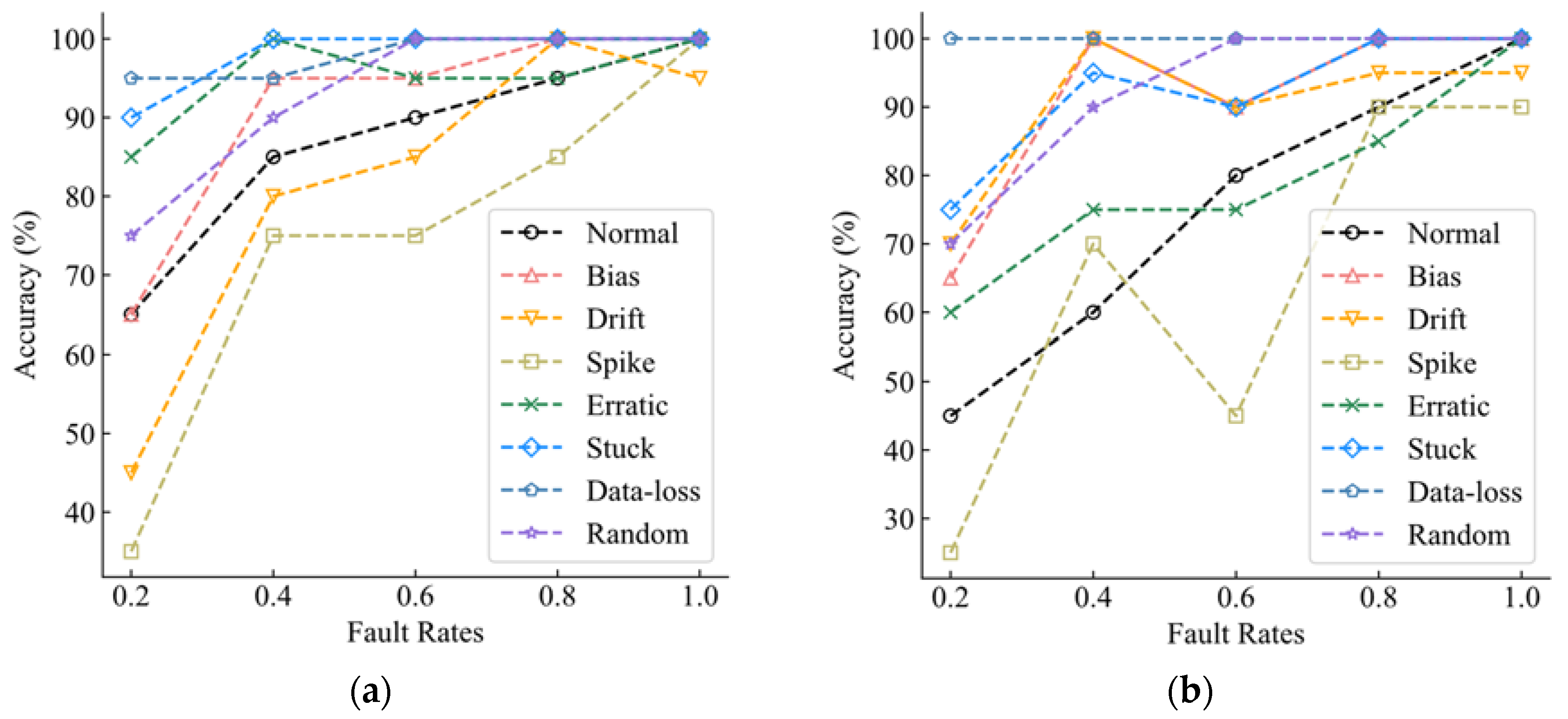
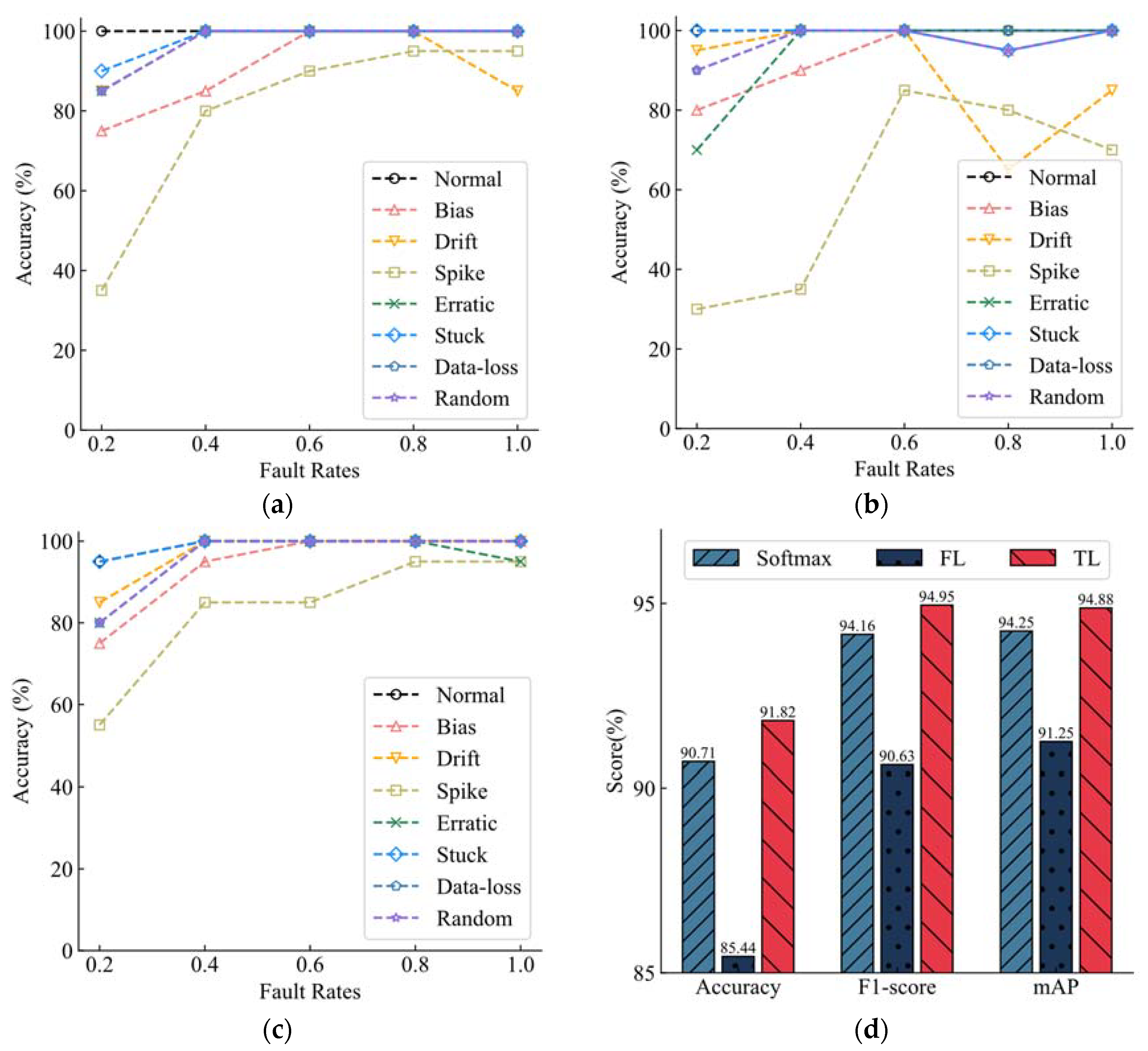
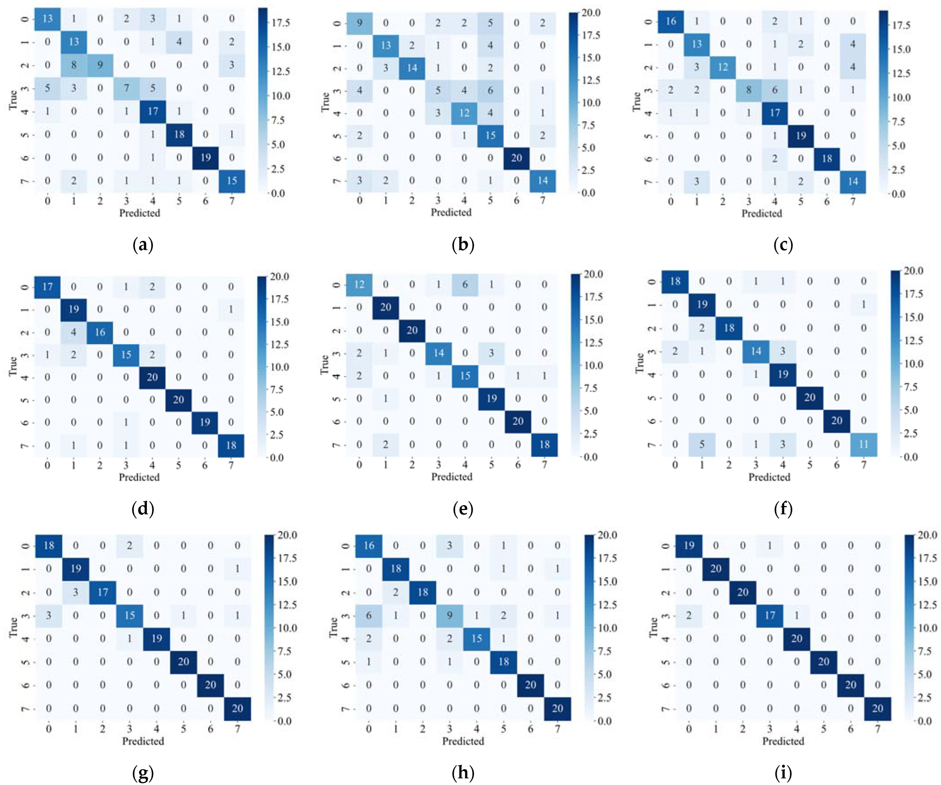
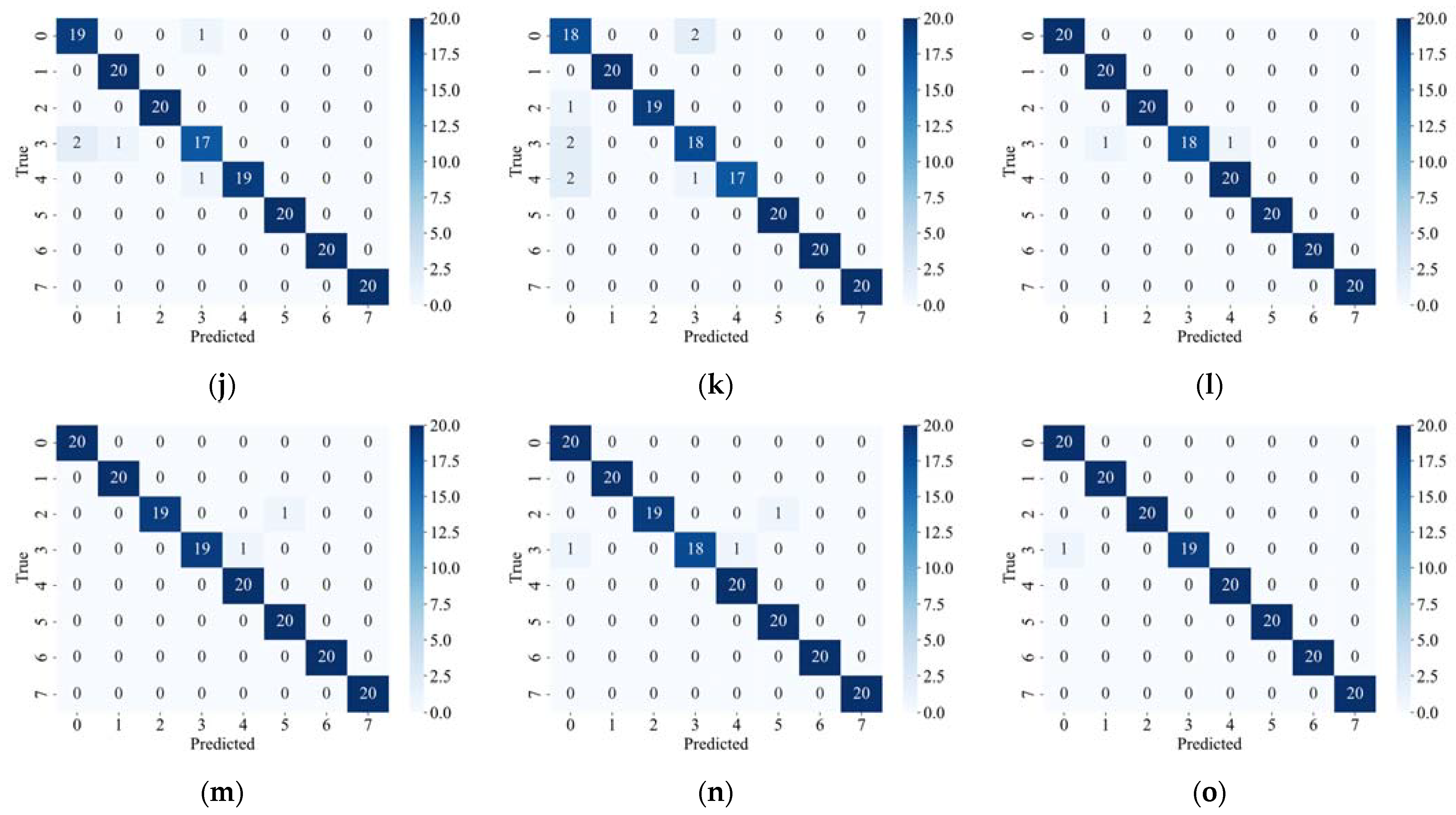
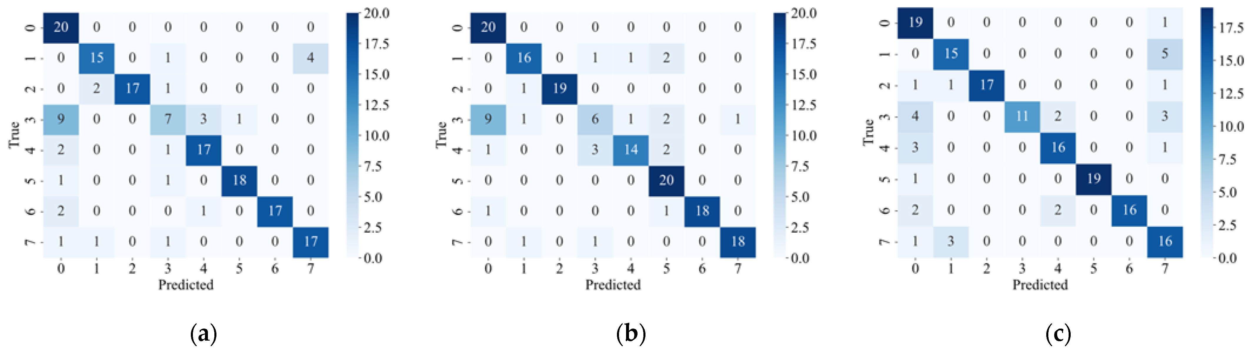
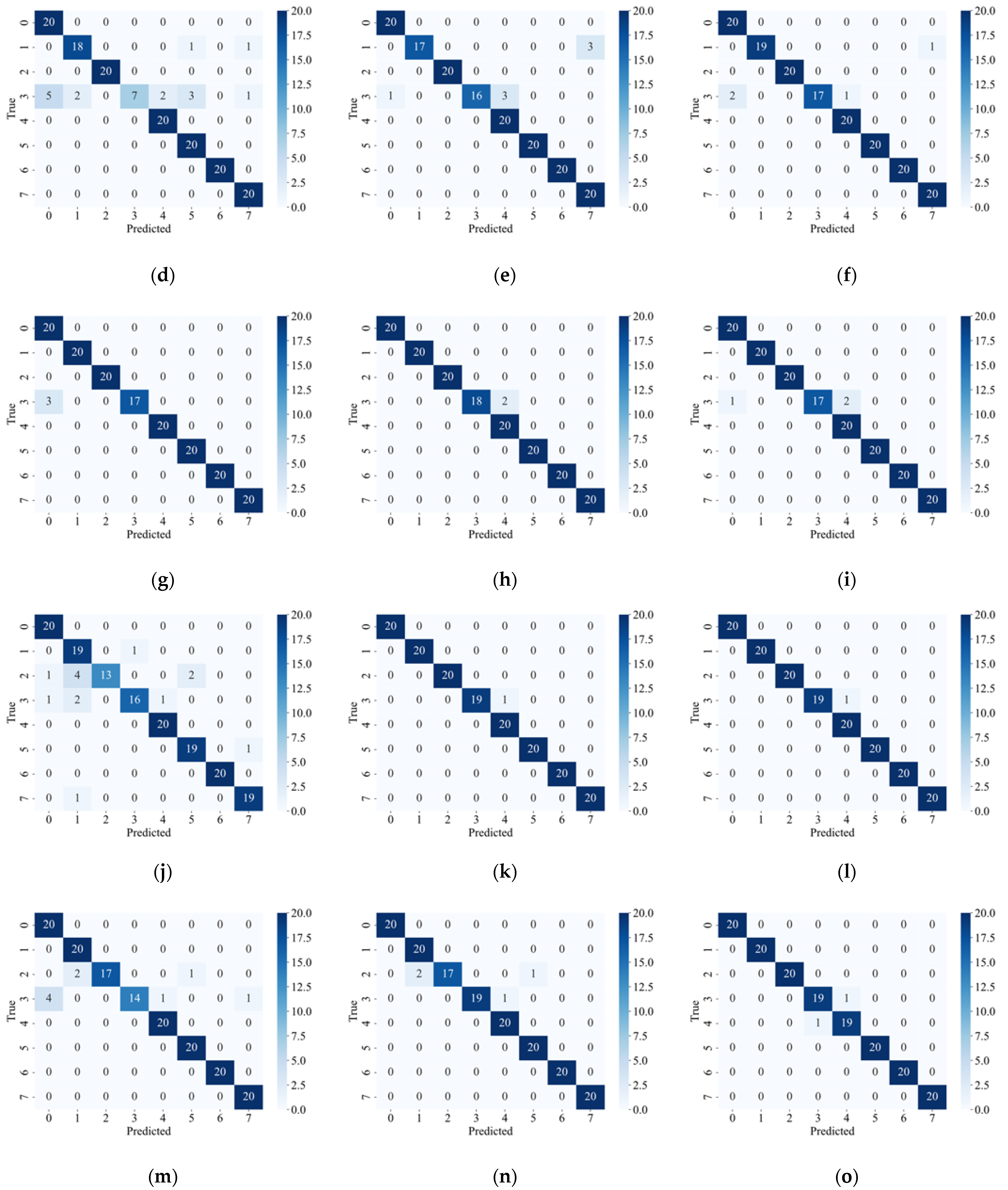
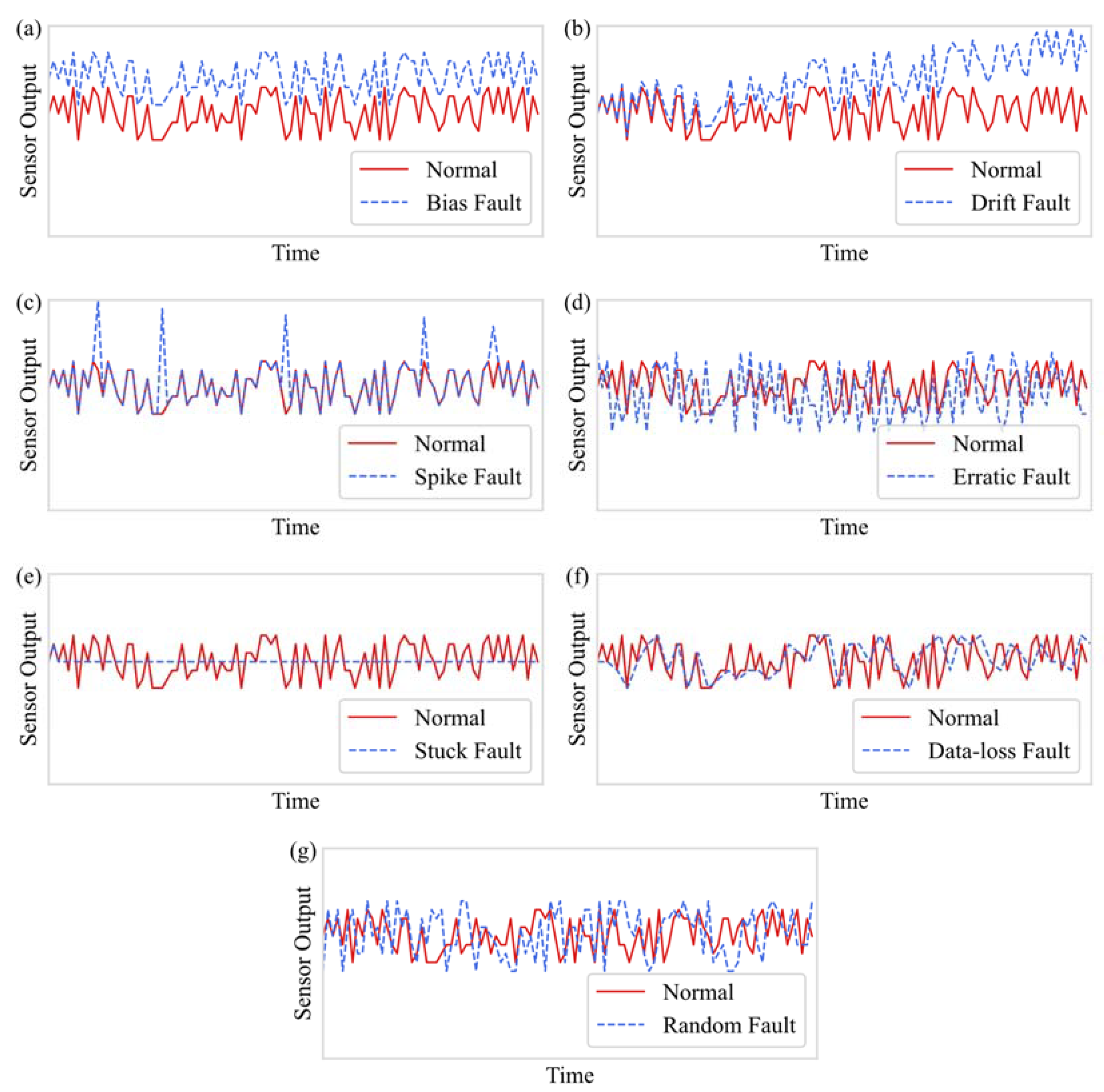
To further illustrate, Figure 6a,b shows the recognition accuracy of the three classifiers for the eight categories under different fault rates. In order to better demonstrate the superiority of the proposed method, Figure 7 shows the confusion matrix of each model under different failure rates. Figure 6a shows the classification accuracy of each fault type in data sets with fault rates of 0.2, 0.4, 0.6, 0.8, and 1 for the model trained using the XGBoost default loss function. It can be seen that the diagnostic accuracy of the model generally increases with the increase of the fault rate, except that the classification performance of the categories Erratic and Drift decreases when the fault rate is 0.6 and 1, respectively. When the fault rate of the model reaches 0.8, the recognition accuracy of all categories reaches more than 80%. When the fault rate reaches 1, the prediction accuracy of other categories of faults reaches 100%, except Drift faults.

Figure 6b shows the model trained with FL as a loss function and the classification accuracy of each fault type in data sets with fault rates of 0.2, 0.4, 0.6, 0.8, and 1, respectively. With the increase in the fault rate, the overall identification accuracy of the model is gradually improved. However, when the fault rate is 0.6, the performance of the model decreases obviously, and the identification accuracy of Spike, Erratic, Stuck, and Drift decreases somewhat, among which the identification accuracy of Spike declines most seriously. This makes the overall recognition of the model decline even less than the model’s recognition accuracy when the fault rate is 0.4, but when the fault rate reaches 0.8, the accuracy of various categories can still reach more than 80%, but the overall classification accuracy of the model is not high. In general, the overall performance of the model trained with FL as a loss function is not as good as that of the model trained with the default loss function, especially when the fault rate is below 0.6. The gap between the two is obvious, and when the fault rate reaches 0.8 and 1, the performance gap between the two is reduced.

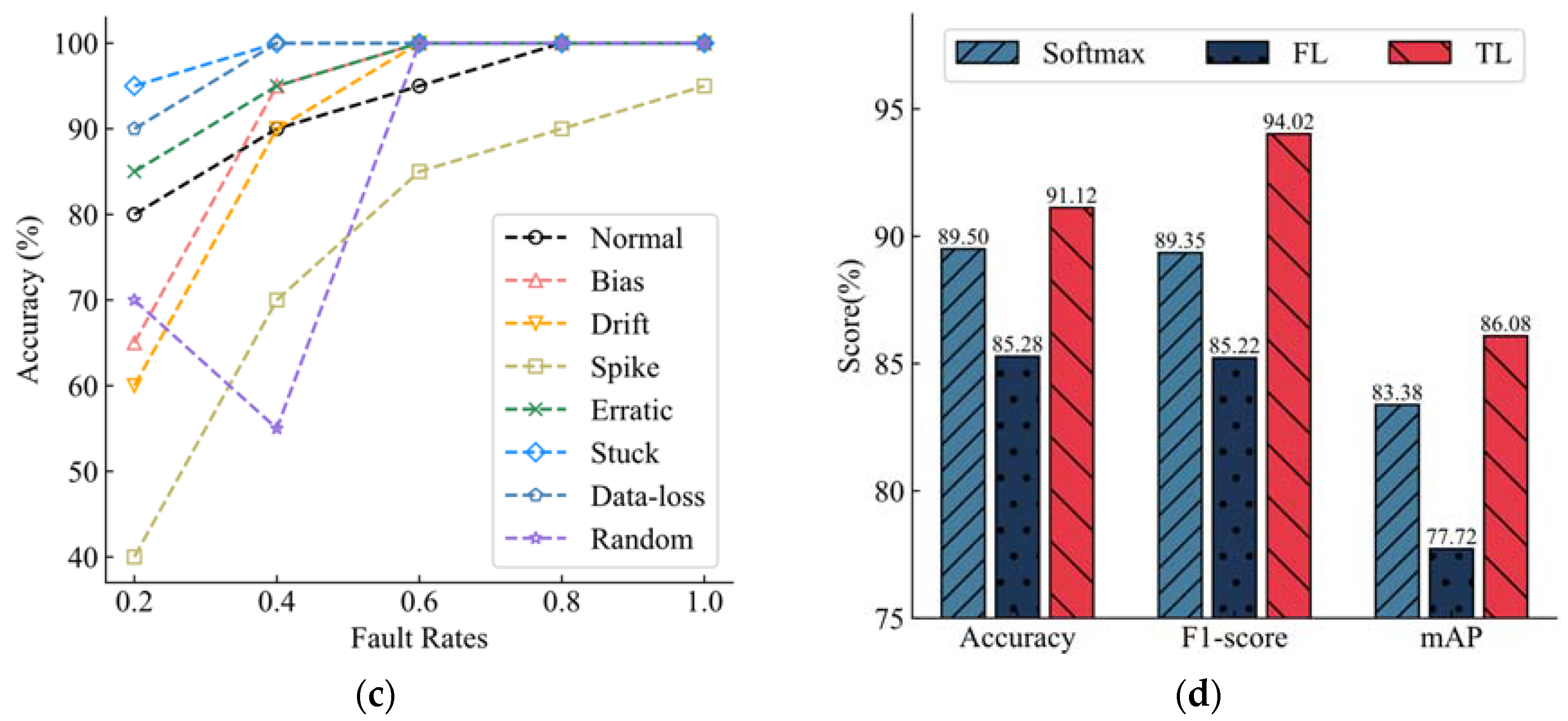
Figure 6c shows the classification accuracy of each fault type in data sets with fault rates of 0.2, 0.4, 0.6, 0.8, and 1 for the model trained with TL. With the increase in the fault rate, the overall recognition accuracy of the model still increases. When the fault rate is 0.4, the classification performance of the model Random decreases, which is also the main factor restricting the recognition accuracy of the model. However, when the fault rate reaches 0.6, the model shows good classification performance, and the accuracy rate of all categories reaches more than 80%. Except for Normal and Spike, the accuracy rate of other categories reaches 100%. When the fault rate reaches 1, in addition to the classification accuracy of Spike faults (but also up to 95%), the identification accuracy of other categories reaches 100%. It can be seen that TL makes the model have higher precision.

The classification of spike faults is a difficult task for XGBoost models, and in this regard, the models do not always do a good job of classifying spike faults, whether they are trained with default loss functions, FL training models, or TL training as loss functions. However, TL-trained models generally have the best performance in identifying spike faults. For the model trained using TL, when the fault rate is 0.4, the recognition accuracy of random faults has a huge decline, which is also the reason why the accuracy of the model trained using TL is not improved but decreased compared with the model trained using the default loss function at this fault rate. Data loss faults and stuck faults are relatively easy tasks for models, and models trained with TL and default loss functions can maintain an at least 90% recognition accuracy. In general, the TL-trained model can improve the accuracy of XGBoost. In addition to the recognition of random faults with a fault rate of 0.4, the model has been improved to varying degrees in other cases.

In addition to accuracy, this study also evaluated the performance of the models using Precision, Recall, F1-score, and mAP metrics.

Table 3. Precision and Recall of classifiers at different fault rates.

Loss Function	Fault Rates
	0.2		0.4		0.6		0.8		1
	Precision	Recall	Precision	Recall	Precision	Recall	Precision	Recall	Precision	Recall
Softmax	0.6938	0.7275	0.9	0.91	0.925	0.9263	0.9688	0.9675	0.9875	0.9875
Focal loss	0.6375	0.6575	0.8625	0.8625	0.8375	0.8413	0.95	0.955	0.9813	0.9813
Triage Loss	0.7313	0.7775	0.8688	0.885	0.975	0.9738	0.9875	0.9875	0.9938	0.9938

and

Table 4. F1-score and mAP of classifiers at different fault rates.

Loss Function	Fault Rates
	0.2		0.4		0.6		0.8		1
	F1-Score	mAP	F1-Score	mAP	F1-Score	mAP	F1-Score	mAP	F1-Score	mAP
Softmax	0.6865	0.5461	0.9007	0.8322	0.9242	0.8692	0.9686	0.9442	0.9875	0.9772
Focal loss	0.6362	0.4933	0.8585	0.7699	0.8342	0.7416	0.9511	0.9157	0.9811	0.9657
Triage Loss	0.7296	0.5974	0.8658	0.7856	0.9746	0.955	0.9873	0.9772	0.9937	0.9886

present the Precision, Recall, F1-score, and mAP of the models trained with three different loss functions at fault rates of 0.2, 0.4, 0.6, 0.8, and 1, respectively. It can be observed that the model trained with TL outperforms the models trained with the default loss function and focal loss in terms of Precision, Recall, F1-score, and mAP, except for the case where the fault rate is 0.4. This indicates that the model trained with TL exhibits a superior performance.

By comparing trained models with the default loss functions and FL, it can be seen that the models trained with TL showed average improvements of 6.73% and 1.81% in classification accuracy, 6.80% and 1.86% in the F1-score, and 10.75% and 3.24% in mAP, respectively, across five different fault rates. The maximum improvements observed at these five fault rates were 16.41% and 5.4% in classification accuracy, 16.83% and 5.45% in the F1-score, and 28.78% and 9.87% in mAP, respectively.

The overall performance of the model is shown in Figure 6d. The average level of the three loss training models under different fault rates is compared. The TL training model has the best performance, and both Accuracy, the F1-score, and mAP have achieved the highest scores. The default loss function training model shows good improvement compared to the FL training model, which improved significantly. XGBoost is a mature algorithm, and using TL as a loss function can still make the model perform better. In order to achieve higher classification accuracy and a better performance of the model, it is recommended to use TL as a loss function to train the model.

4.2. Experiments Were Performed on the Public Dataset

4.2.1. Data Acquisition

The experiment was conducted using a publicly available gearbox dataset from Southeast University in China, which was collected from the Drivetrain Dynamics Simulator. Each file has eight channels of signal. In order to be consistent with the previous experiment, the data of channel three were selected for the experiment, that is, the vibration data of the planetary gearbox in the y direction and 350,000 consecutive data were selected, and the data were amplified to the same scale as the previous experiment, as shown in Figure 8. Similarly, seven common sensor faults were injected into the original signal in different proportions to obtain five fault rates and eight state data, including the normal state. Then, each group of data was divided into 70 samples to obtain a data set of 5 × 8 × 70 × 5000, in which 5 × 8 × 50 groups of data were used for training, and 5 × 8 × 20 groups of data were used for testing. The hyperparameters used in the training model are also consistent with the previous experiment.

4.2.2. Experimental Result

The accuracy of the model trained with the three loss functions under different fault rates is shown in

Table 5. Accuracy of models trained with different loss functions under different fault rates.

Loss Function	Fault Rates
	0.2	0.4	0.6	0.8	1
Softmax	0.8	0.95625	0.9875	0.99375	0.975
Focal Loss	0.81875	0.90625	0.98125	0.9125	0.94375
Triage Loss	0.80625	0.975	0.98125	0.99375	0.9875

. The model trained with the default loss function achieves the highest accuracy when the fault rate is 0.6 and 0.8. The model trained with FL achieved the highest accuracy when the fault rate was 0.2. The TL-trained model achieved the highest recognition accuracy at fault rates of 0.4, 0.6, and 0.8. In general, the model trained using TL had the best effect, achieving the highest recognition accuracy in the three fault rates and achieving the second highest accuracy in the absence of the highest accuracy.

To further illustrate, Figure 9a–c respectively shows the classification accuracy of the model trained with three loss functions at different fault rates. In order to better demonstrate the superiority of the proposed method, Figure 10 shows the confusion matrix of each model under different failure rates. Figure 9a shows the classification accuracy of the model trained using the default loss function for each category at five fault rates. It can be seen that with the increase in the fault rate, the overall accuracy of the model will increase, except for the recognition accuracy of the Drift category which decreases when the fault rate is 1. When the fault rate reaches 0.4, the recognition accuracy of the model for each category reaches more than 80%, and the recognition accuracy of other categories reaches 100%, except for Bias and Spike.

Figure 9b shows the recognition accuracy of each category for a model trained using FL as a loss function under five fault rates. When the fault rate of the model is 0.8, the recognition accuracy decreases significantly, which is mainly reflected in the decline of the recognition accuracy of the Drift, Spike, Bias, Erratic, and Random categories. The model performs best when the fault rate is 0.6. The recognition accuracy of the Spike category is 80%, and the recognition accuracy of other categories reaches 100%.

Figure 9c shows the recognition accuracy of each category for the model trained using TL as a loss function under five fault rates. With the increase in the fault rate, the overall recognition accuracy of the model increases, except that when the fault rate is 1, where the recognition accuracy of the Erratic category decreases. After the fault rate reached 0.4, the model had a good performance, and the overall recognition accuracy rate came to more than 85%. It can be seen that using TL to train the model can make the model perform well.

The recognition of Spike classes remains the most difficult task for XGBoost models of all classes, and the three loss-function-trained models always perform the worst on the recognition of Spike classes. The FL-trained model performed very erratically at a fault rate of 0.8, with a decline in the recognition accuracy for many categories, and performed relatively poorly except at a fault rate of 0.2. Models trained using the default loss function and TL performed relatively well, with a good recognition accuracy for each category at various fault rates.

Table 6. Precision and Recall of classifiers at different fault rates.

Loss Function	Fault Rates
	0.2		0.4		0.6		0.8		1
	Precision	Recall	Precision	Recall	Precision	Recall	Precision	Recall	Precision	Recall
Softmax	0.8	0.8188	0.9563	0.9613	0.9875	0.9888	0.9938	0.9938	0.975	0.9763
Focal loss	0.8188	0.8263	0.9063	0.9188	0.9813	0.9838	0.9125	0.9225	0.9438	0.9488
Triage Loss	0.8063	0.8488	0.975	0.9763	0.9813	0.9825	0.9938	0.9938	0.9875	0.9875

and

Table 7. F1-score and mAP of classifiers at different fault rates.

Loss Function	Fault Rates
	0.2		0.4		0.6		0.8		1
	F1-Score	mAP	F1-Score	mAP	F1-Score	mAP	F1-Score	mAP	F1-Score	mAP
Softmax	0.7967	0.6912	0.9555	0.9232	0.9875	0.9777	0.9937	0.9886	0.9746	0.9549
Focal loss	0.8082	0.715	0.8902	0.8382	0.9811	0.9673	0.9105	0.851	0.9413	0.9007
Triage Loss	0.8109	0.704	0.9746	0.9549	0.9809	0.9663	0.9937	0.9886	0.9875	0.9772

show the Precision, Recall, F1-score, and mAP of the three loss-function-trained models under five fault rates. Among the 20 comparisons, the TL-trained model achieved the highest score of 14, the default loss function and FL-trained model achieved the highest scores of 4 and 2, respectively. So, in general, training a model using TL as a loss function results in a better performance.

The overall performance of the model is shown in Figure 9d. The average level of the three loss training models under different fault rates is compared. Among them, the TL training model still has the best performance, with the highest scores in the Accuracy, F1-score, and mAP. The model trained with FL had the worst performance, and compared with the model trained with the default loss function, the effect decreased rather than increased, and the decline was serious.

Experiments were conducted on the bearing (self-measured) dataset and the gear (public) dataset to demonstrate that the proposed method performs better when processing different types of vibration data. The results indicate that the model trained using TL has better performance when dealing with two common vibration data.

5. Conclusions

Using TL as the loss function and inputting data into XGBoost for training, this paper proposed a VSFD method, targeting the common types of faults in vibration sensors. In the process of model training, it is important to prevent the loss of the model from being overwhelmed by a large number of basic negative classes, so TL is designed as a loss function to train the model. By scaling the CE, the loss of difficult samples is increased so that the model prioritizes challenging samples, resulting in an improved classification performance. The method was applied to the published gearbox vibration data set and the fault diagnosis experiment of a bearing vibration sensor on a low-speed and heavy-load test stand and compared with the default loss function and FL. According to the findings, whether testing with the public dataset or using an experimental dataset, the accuracy of the model trained with TL is outstanding, and it is better than the model using default loss and FL training in the evaluation index of the F1-score and mAP model.

First of all, this paper proposed a VSFD method based on XGBoost to identify seven common faults of vibration sensors. This method shows high accuracy, with an average accuracy of more than 90% under different fault rates. Secondly, as simple negative classes occupy most of the iterative process of the model in the training process of samples with unbalanced categories, this paper designs a new loss function TL to train the model. This will help the model focus more on difficult samples and have a higher classification accuracy and performance. Finally, the methodology has been utilized in conducting the fault diagnosis experiment of the bearing vibration sensor on a low-speed and heavy-load test stand. The results of the experiment indicate that when compared to the model trained using FL and the default loss function, the model trained using TL, the classification accuracy is improved by 16.41% and 5.4%, the F1-score is improved by 16.83% and 5.45%, and mAP is improved by 28.78% and 9.87%.