On-Line Application of SHEM by Particle Swarm Optimization to Grid-Connected, Three-Phase, Two-Level VSCs with Variable DC Link Voltage

Abstract

This paper is devoted to an otablen-line application of the selective harmonic elimination method (SHEM) to three-phase, two-level, grid-connected voltage source converters (VSCs) by particle swarm optimization (PSO). In such systems, active power can be controlled by the phase shift angle, and reactive power by the modulation index, against variations in the direct current (DC) link voltage. Some selected, low-odd-order harmonic components in the line-to-neutral output voltage waveforms are eliminated by calculating the SHEM angle set continuously through the developed PSO algorithm on field-programmable gate array (FPGA)-based computing hardware as the modulation index is varied. The use of powerful computing hardware permits the elimination of all harmonics up to 50th. The cost function of the developed PSO algorithm is formulated by using an optimum number of particles to obtain a global optimum solution with a small fitness value in each half-cycle of the grid voltage and then updating the SHEM angle set at the beginning of the next full-cycle. Since the convergence of the solution to a global minimum point depends upon the use of correct initial values especially for a large number of SHEM angles, a generalized initialization procedure is also described in the paper. Theoretical results are verified initially using hardware co-simulation. They are also tested using a small scale photovoltaic (PV) supply prototype developed specifically for this purpose. It is demonstrated that the 5th, 7th, 11th, 13th, 17th, and 19th sidekick harmonics are eliminated by on-line calculation of seven SHEM angles through the developed PSO algorithm on a moderately powerful XEM6010-LX150, USB-2.0-integrated FPGA module. All control and protection actions and the calculation of SHEM angles are achieved by a single FPGA chip and its peripherals within the FPGA board.

1. Introduction

Various modulation schemes have been employed in inverter circuits, such as space vector modulation (SVM), pulse width modulation (PWM), and the selective harmonic elimination method (SHEM). The main feature of the SVM scheme is the fast dynamic response obtained, whereas the SHEM has superior harmonic performance for a given switching frequency. The performance of the best PWM modulation techniques is somewhere between the SVM and SHEM [1]. On-line application of SHEM to voltage source converters (VSCs) for the elimination of low-order output voltage harmonics, however, has not been reported yet in the literature due to the computational overhead of the digital implementation on processors.

In grid-connected VSCs of either two-level or multilevel types, the SHEM angles can be determined by solving a set of nonlinear algebraic equations. The resulting mathematical model contains sinusoidal terms and the number of equations in the model is equal to the number of switching angles. Two main groups of techniques have been presented in the literature to solve these nonlinear equations. Iterative methods, such as the Newton–Raphson method [2,3] and the homotopy algorithm [4,5,6,7], are given in the first group. Some other iterative numerical techniques have been proposed in [8,9,10,11], and the Walsh-function-based analytical technique has been adopted in [12]. In [13,14], to find the solutions for all modulation indices, theories of resultants and symmetric polynomials have been employed, which are then used to solve the polynomial equations obtained from transcendental equations. It has been shown in [13] that such SHEM equations do not have a solution set for some unfeasible modulation index values of the inverter.

In the second group, SHEM is considered as an optimization problem, which is investigated through evolutionary search algorithms. Evolutionary search algorithms have been used to solve various industrial problems in recent years. Easier solutions can be found to these problems by this way as compared to the analytical methods, and in some cases, they constitute the unique way to find a feasible solution [15]. The global optimum solution can be found by these algorithms for complete elimination of certain harmonics or optimum switching angles can be offered in cases where a feasible solution cannot be found. Some major evolutionary search algorithms which have been applied can be cited as the genetic algorithm (GA) [16,17,18], particle swarm optimization (PSO) [2,19,20], ant colony optimization [21], the bee algorithm [22], and the bacterial foraging algorithm [23].

Until now, SHEM has been applied off-line in industry applications of grid-connected converters by using lookup tables (LUTs). Among these, distribution-type, two-level static synchronous compensator (STATCOM) systems based on a current source converter (CSC) with a variable direct current (DC) link current are reported in [24,25,26], two-level voltage source converter (VSC)-based distribution-type STATCOM systems with variable DC link voltages in [27], and a transmission-type cascaded multilevel converter-based STATCOM system with constant DC link voltage in [28,29]. On the other hand, VSCs with variable DC link voltages are widely used in photovoltaic (PV) and traction applications, in which the modulation index value for the VSC changes in a wide range as the DC link voltage varies. In such applications, the off-line SHEM using LUTs for determination of switching angle sets is disadvantageous primarily due to the stepwise control of the modulation index value resulting in minimization of selected harmonics instead of their elimination, and secondarily due to the infeasible region of the solution space [30] and the need for a large LUT storage area [31].

To solve these problems, researchers have searched for an effective way to apply SHEM on-line in order to allow for continuous control of SHEM angles. The generalization ability of an artificial neural network (ANN) has been applied in [30] to cope with this problem. The switching angles have been calculated beforehand for different DC source values using GA, then the switching angles have been determined for different DC link voltage magnitudes at each phase of the multilevel inverter in real-time by adopting the ANN to train the controller. By this way, the ANN can be used instead of a LUT, thus introducing its inherent capability to generalize the solution space into the problem with proper training. In [31], another approach was investigated for on-line applications of SHEM, where an analytical procedure was employed for computation of all pairs of valid switching angles in five-level, H-bridge cascaded inverters. Here, a fully analytical calculation is allowed for the switching angles using Chebyshev polynomials and Waring equations. This procedure can be implemented in real-time using either a digital signal controller, a programmable logic device, or a field-programmable gate array (FPGA), as claimed in [31], due to its limited complexity. On the other hand, digital control techniques applied to voltage source inverters in renewable energy applications were reviewed in [32]. On-line optimal switching frequency selection for grid-connected voltage source inverters was presented in [33].

In this paper, calculation of SHEM angles in real-time is described by using a PSO algorithm, specifically developed for this purpose, and a digital computing hardware. An on-line application of SHEM is important especially for grid-connected inverters with variable DC link voltages in order to eliminate all odd-order characteristic power system harmonics up to the 50th. The initialization procedure for the PSO algorithm is generalized to ensure the convergence of the solution to a global optimum by assuming that the modulation index, and hence the inverter’s output voltage, is initially zero. A timing diagram for the on-line application of SHEM is given in the paper, in which the number of SHEM angles, up to 17, is calculated in each half-cycle of the supply voltage waveform, and the firing instants of all power semiconductors of the grid-connected inverter are updated in the next full-cycle. Keeping the switching pattern constant in each full-cycle avoids the generation of DC component and even-order voltage harmonics. The proposed method is verified by a hardware co-simulation work, and the theoretical results are justified in the field on a small-size photovoltaic (PV) supply by calculating on-line seven SHEM angles on a moderately powerful FPGA board. In the prototype PV supply, active power control is implemented by phase shift angle control, reactive power control by variation of the modulation index, and elimination of selected sidekick voltage harmonics (5th, 7th, 11th, 13th, 17th, and 19th) in the inverter’s output phase voltage by SHEM.

2. Problem Description

2.1. Possible Application Areas of SHEM

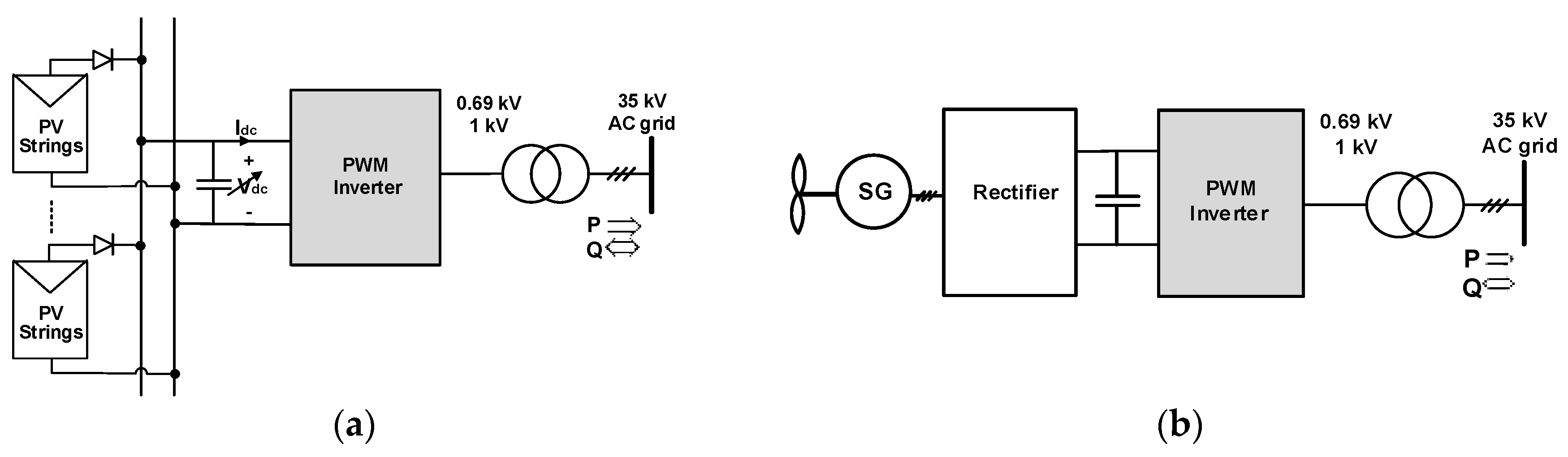
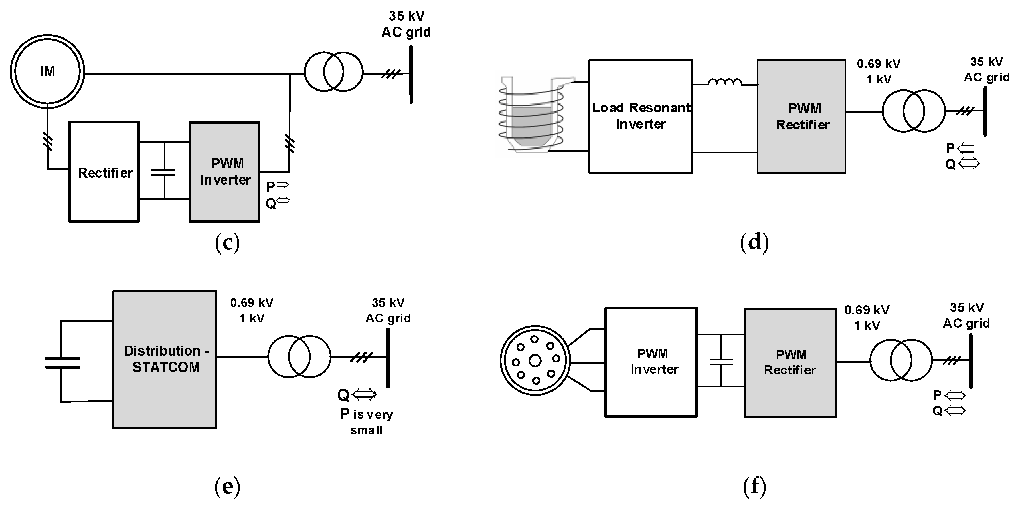
Possible application areas of SHEM are summarized in Figure 1. The common properties of these applications are: (i) few MVA apparent power rating, (ii) Connection to an available three-phase, medium-voltage grid bus though a dedicated coupling transformer, and (iii) 690 V or 1 kV voltage rating for the grid-side VSC. The application of SHEM is suitable for the gray-shaded converters in Figure 1. In these three-phase, two-level VSCs, either high voltage insulated gate bipolar transistor (HV-IGBT) type or integrated gate commutated thyristor (IGCT) type power semiconductors are used in practice. IGBTs and IGCTs in these converters can be switched, respectively, in the range of 1.5 kHz and 500 Hz in practical applications because of their relatively high switching losses. SHEM best matches the needs of such applications, i.e., minimum harmonic current distortion on the grid side and high conversion efficiency. In the near future, with the advents in SiC power MOSFET technology, these new power semiconductors can be switched at much higher frequencies in such applications. In the systems shown in Figure 1a–c, the DC link voltage is variable depending upon the operating condition. In the system in Figure 1d, the DC link voltage may be kept constant or varies in a narrow range. However, in the systems in Figure 1e,f, the DC link voltage may be varied only for performance concerns.

In most of these applications, the grid-side inverter or rectifier is connected to the grid by using a dedicated coupling transformer as shown in Figure 1. If the leakage reactance of the coupling transformer is not sufficiently large for minimization of total demand distortion (TDD), a small series inductor bank may be connected on the converter side of the system. On the other hand, for small-size systems, the grid connection is achieved by using an LCL filter or its derivatives, since an inductance-only filter is not sufficient to suppress high-order harmonic components which are not eliminated by SHEM.

2.2. Switching Techniques for SHEM

Various switching techniques that can be used in the application of SHEM are clearly described in [34]. Line-to-line converter voltage harmonics can be directly eliminated by the three-phase line-to-line technique (TLL), and line-to-neutral converter output voltage harmonics by the three-phase line-to-neutral techniques (TLN1 and TLN2). In the TLL technique, a 2 times higher switching frequency and a higher DC link voltage are required in comparison with those of the TLN2 technique in order to eliminate the same number harmonics and to give the same grid voltage. Similar conclusions can be drawn also for the TLN1 technique. 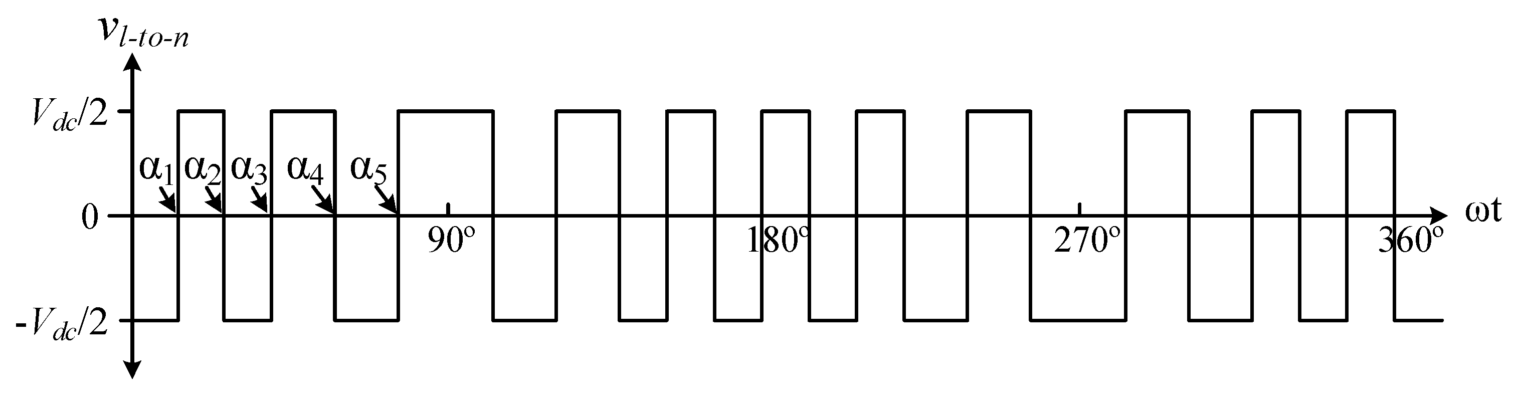In view of PV applications with direct power conversion, the TLN1 and TLN2 techniques are more suitable to maintain the maximum power-point voltage, V_mpp, and hence the DC link voltage of the inverter within an acceptable range, e.g., 600–900 V for thin-film PV arrays. On the other hand, TLN1 differs from the TLN2 technique by the number of harmonics to be eliminated from the voltage waveform. This number is even for the TLN1 technique, whereas it is odd for the TLN2 technique. It can be examined from the line-to-neutral voltage waveform in Figure 2 that an odd number of notch angles α₁ to α₅ exists, resulting in the elimination of an even number of characteristic power system harmonics, i.e., the 5th, 7th, 11th, and 13th in the line-to-neutral voltage waveform. In SHEM, the first notch angle is always used to control the fundamental voltage component. Triplen harmonics, such as the 3rd, 9th, and 15th, will be cancelled out in line-to-line voltage waveforms although they are present in line-to-neutral voltage waveforms. There will be no even-order characteristic power system harmonics, such as the 2nd, 4th, 6th, 8th, etc., in line-to-neutral voltage waveforms because of the quarter-wave odd symmetry [24,27,35,36]. The converter’s switching frequency f_c can be expressed as in (1) for TLN1 and TLN2 techniques:

$$f_c=(2N+1)f_1\{\begin{array}{c}N\mathrm{is}\mathrm{odd}\mathrm{for}\mathrm{TLN}1\\ N\mathrm{is}\mathrm{even}\mathrm{for}\mathrm{TLN}2\end{array}$$

(1)

where, f₁ is the frequency of the fundamental component and N the total number of harmonics to be eliminated, including the fundamental component to be controlled.

If TLN2 were chosen, a higher-order harmonic component, the 13th for N = 4 or the 19th for N = 6 among the sidekick harmonics (the 11th and 13th for N = 4 or the 17th and 19th for N = 6) could not be eliminated. Therefore, in this research work, the TLN1 technique is preferred.

The Fourier series expansion of the line-to-neutral voltage waveform in Figure 2 gives the magnitude of the nth characteristic power system harmonic, $b_n$, obtained from (2).

$$b_n=\frac{4}{n\pi }\frac{V_{dc}}{2}\left[-1-2{\displaystyle \sum _{k=1}^N{(-1)}^k\cos (n{\alpha }_k)}\right]$$

(2)

where, n is the odd harmonic order, V_dc the DC link voltage, and α_k the switching angle for k = {1, 2, …, N}.

N transcendental equations with N unknowns (α₁, α₂, …, α_N) in (3) are then obtained by setting the fundamental voltage component to a prespecified value and equating the remaining N − 1 harmonics all to zero.

$$\left[\begin{array}{cccc}2\cos ({\alpha }_1)& -2\cos ({\alpha }_2)& \cdots & 2{(-1)}^{N+1}\cos ({\alpha }_N)\\ 2\cos (5{\alpha }_1)& -2\cos (5{\alpha }_2)& \cdots & 2{(-1)}^{N+1}\cos (5{\alpha }_N)\\ ⋮& ⋮& \ddots & ⋮\\ 2\cos (X{\alpha }_1)& -2\cos (X{\alpha }_2)& \cdots & 2{(-1)}^{N+1}\cos (X{\alpha }_N)\end{array}\right]=\left[\begin{array}{c}1+\frac{\pi b_1}{2V_{dc}}\\ 1\\ ⋮\\ 1\end{array}\right]$$

(3)

where X = 3N − 2 and α constraints $0<{\alpha }_1<{\alpha }_2<\cdots <{\alpha }_N<\frac{\pi }{2}$.

A simultaneous solution of the set of transcendental equations in (3) is necessary to obtain a solution set for α₁ to α_N. Since these equations are nonlinear, either an iterative method or an evolutionary search algorithm is required.

2.3. Need for On-Line SHEM

The technical specifications of a three-phase, two-level, and grid-connected VSC with some selected harmonics eliminated by SHEM are assumed to be as follows.

• It provides conversion of the desired amount of DC power to AC over a wide DC link voltage range, e.g., V_dc = 600 V to 900 V for the thin-film PV systems in Figure 1a.
• Active power control is achieved by controlling the phase shift angle, δ, of the VSC output voltage with respect to the supply voltage.
• The reactive power generated or consumed by the VSC should be adjusted to any prespecified value by varying the magnitude of the VSC’s output voltage by controlling the modulation index over the entire operating range.

The need for on-line SHEM is justified by carrying out two case studies as given below.

Case Study I: Constant SHEM Angle Set with Variable DC Link Voltage

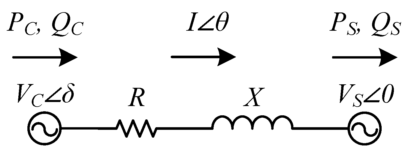
The three-phase, grid-connected VSC can be represented by the single-line diagram shown in Figure 3.

The output series filter reactor’s internal resistance component, R, and/or the coupling transformer’s leakage impedance is much smaller than the inductive reactance component, X, and phase-shift angle, δ, between the fundamental component of converter voltage, V_c, and the fundamental component of supply voltage, V_s, phasors is very small, then sinδ ≈ δ and cosδ ≈ 1 [27,36]. Under these assumptions, the active and reactive powers generated by the VSC, (P_c, Q_c), and active and reactive powers consumed by the grid, (P_s, Q_s), can be approximated by expressions in (4) to (6).

$$P_C\cong P_S\cong 3\frac{V_C{V}_S}{X}\delta$$

(4)

$$Q_C\cong 3V_C\frac{V_C-V_S}{X}$$

(5)

$$Q_S\cong 3V_S\frac{V_C-V_S}{X}$$

(6)

Since V_s and X in (6) are constant, Q_s can be adjusted to any preset value only by controlling V_c. The relationship between the rms value of the fundamental component of the VSC’s output voltage, V_c, and the variable DC link voltage, V_dc, is given by the modulation index expression in (7). Since M is kept constant for a constant SHEM angle set, as V_dc changes there will be no control on V_c and hence on Q_s. Therefore, the use of constant SHEM angles in the control system of grid-connected inverters with variable DC link voltages is to be avoided.

$$M=\frac{\pi {\widehat{V}}_c}{2V_{dc}}=\frac{\pi \sqrt{2}{V}_c}{2V_{dc}}$$

(7)

Case Study II: Off-line SHEM by the Look-Up Table Method

In order to avoid the drawbacks of constant SHEM angles in the reactive power control of grid-connected inverters with variable DC link voltages, M and hence V_c should be adjusted by using several sets of SHEM angles as V_dc changes. The common approach to this problem is the computation of several SHEM angle sets and their storage in an internal or external random access memory (RAM)/read-only memory (ROM) in the form of (a) LUT(s). This approach makes necessary the discretization of M control range into d number of steps for N number of total harmonics to be controlled over the entire operation range of the resulting system, which yields a d × N LUT. Since M and hence SHEM angles α₁ to α_N are controlled stepwise instead of by on-line continuous control, the required value of M at any particular operating point will be rounded to the nearest M number stored in the LUT. This may result in a significant error in V_c and hence Q_s values when the row number, d, of the LUT is kept low. Therefore, d should be as high as possible. A d × N LUT will be impractical if a huge number of harmonics is to be eliminated.

The effects of the order of a LUT on the discretized values of M, the corresponding V_c, and Q_s for unity power factor operation are examined by considering 5 × 7 and 41 × 7 LUTs and the associated results are given in

Table 1. Errors in Reactive Power Adjustment Arising From Off-line SHEM Based on the Look-Up Table (LUT) Method for Unity Power Factor (PF) Operation.

Parameter	Off-Line SHEM				On-Line SHEM
	5 × 7 LUT		41 × 7 LUT
Vdc (V)	600	900	600	900	600	900
M (required)	0.852	0.568	0.852	0.568	0.852	0.568
M (realized)	0.9	0.6	0.85	0.57	0.852	0.568
VC (Vrms, l−n)	243.1	243.1	229.6	230.9	230	230
QS (VAr)	2877	2877	−88	198	0	0
Ps (W)	1350	1675	1350	1675	1350	1675
δ (°)	1.449	1.797	1.534	1.892	1.531	1.900

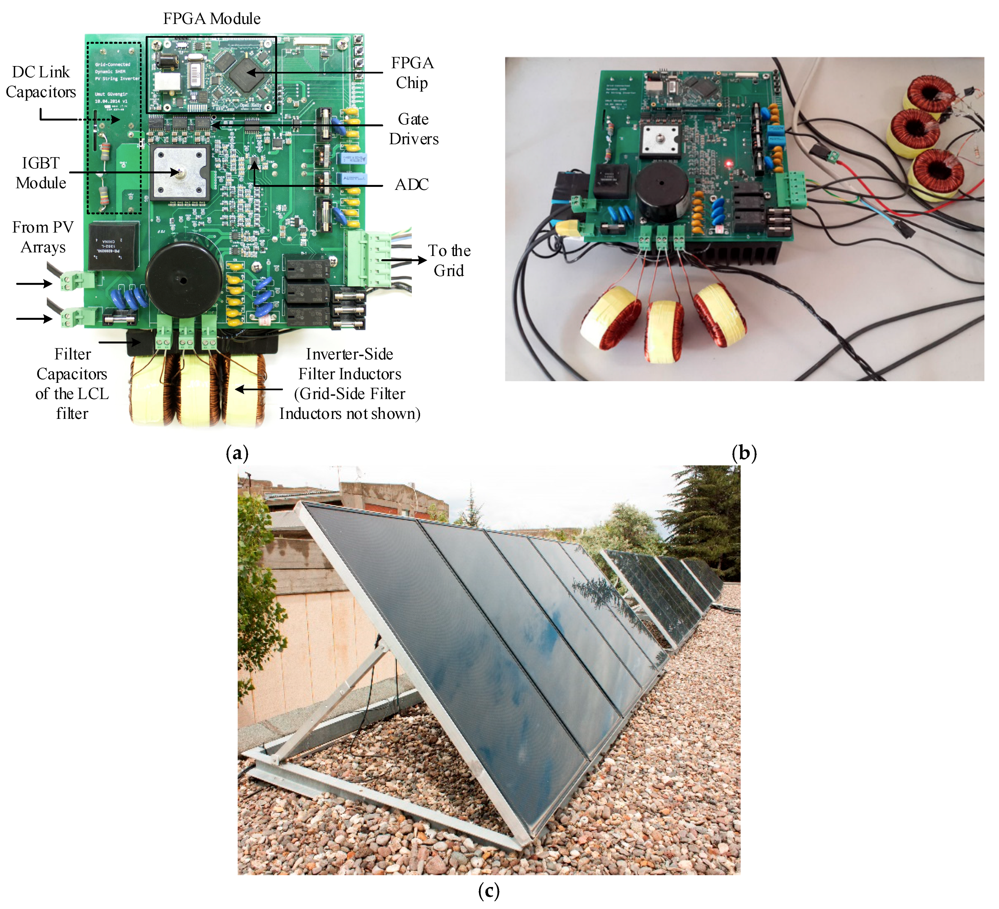
for two different values of DC link voltage (V_{dc (min)} = 600 V, V_{dc (max)} = 900 V, and X = 3.14 Ω at 50 Hz). In this paper, theoretical results are verified on a sample small-scale PV system as described in Section 4. This small-scale prototype is connected to a 400-V, 50-Hz grid. The performance of real-time SHEM in adjusting M, and hence V_c to its set value of 230 V in order to bring Q_s = Q_s(set) to zero is also given in Table 1 for the same problem. As can be understood from the results marked by red colored values in Table 1, V_c and Q_s deviate significantly from their set values in the case of a small-sized LUT. Deviations from the set values can be significantly lowered as the size of the LUT increases (marked by yellow color in Table 1). In order to alleviate the problem arising from the discrete LUT method in variable DC link voltage applications, linear interpolation can be used between consecutive M steps.

At the present time, with the advances in digital electronics area by using a powerful FPGA module or parallel computing hardware, such as a Graphical Processing Unit (GPU), enormously large SHEM angles can be calculated on-line to control M continuously. The performance of the on-line SHEM by using a single FPGA module to control seven harmonics is also given in Table 1 by the green-colored area.

3. Application of PSO to SHEM

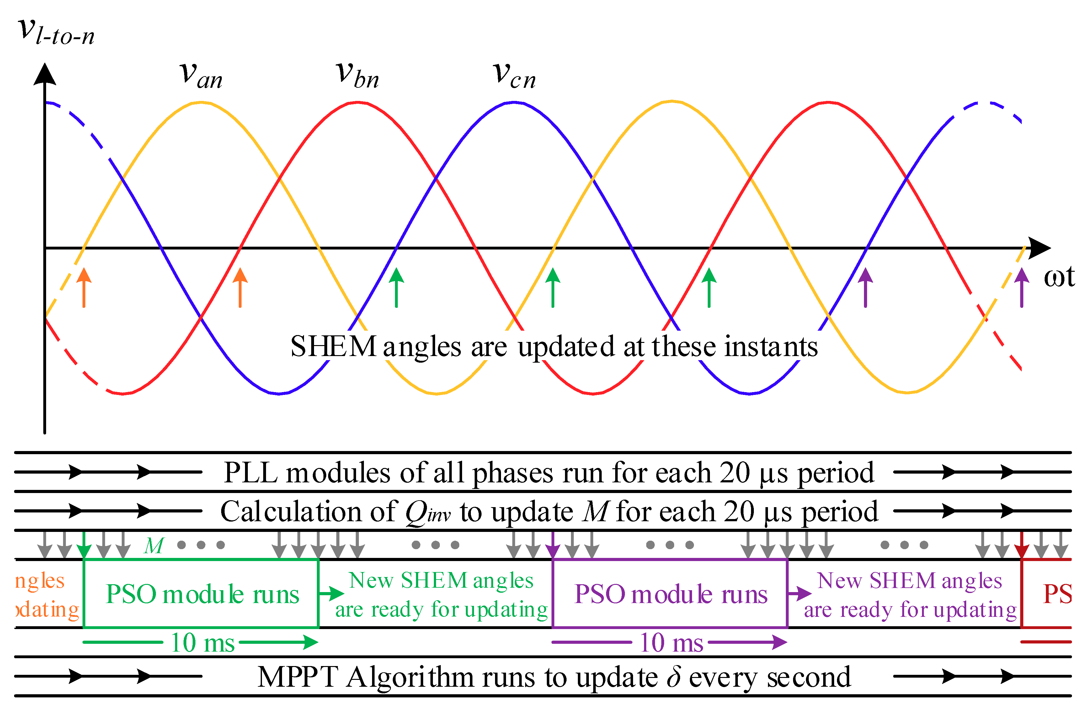
In grid-connected PV inverter applications, since the supply frequency is constant (f₁ = 50 or 60 Hz), SHEM angles should be updated once in a full-cycle (20 or 16.67 ms) with 2π/3 and 4π/3 phase-shifted signals for the remaining two phases. Therefore, on-line calculation of SHEM angles should be carried out in a total execution time less than a period of grid voltage, i.e., 20 ms for 50 Hz applications. However, variable-frequency alternating current (AC) motor drive applications need lower calculation times when the applied motor frequency is higher than the rated frequency. In this research work, the equations in (3) will be solved by the PSO technique, which is an evolutionary search algorithm.

In order to evaluate the fitness values of each particle at each time frame, a cost function should be formulated as required by the PSO. SHEM equations should be put into a format so that each particle is assigned a real fitness value. Then, boundaries of the solution space are defined, and an initial population of swarms is generated in this solution space. Finally, PSO parameters are set, so that the PSO algorithm is ready to find a feasible global optimum to the optimization problem.

3.1. Particle Swarm Optimization (PSO)

The stochastic population-based optimization technique called particle swarm optimization (PSO) has been developed by Dr. Russell Eberhart and Dr. James Kennedy in 1995 [37]. It is initialized with a random or heuristic population which consists of particles such as birds, fish, and insects. Each particle in this research work is a vector composed of seven SHEM angles and in order to assess whether it can be a potential global solution or not, it is evaluated with a fitness function. The particles search the problem space via cognitive and social interaction by pursuing the current optimum particles. The personal best location (pbest) is defined as the coordinates of the particle which is associated with the best personal fitness value acquired so far. The global best location (gbest), however, is defined as the location with the best fitness value which all of the population has reached. In each time frame, each particle updates its velocity towards its pbest and gbest locations. Separate random numbers [38] are employed to weight the total acceleration terms of local and global searches. The velocity, v_i, and position, x_i, update equations are as given in (8) and (9), respectively.

$$v_i(t+1)=K\times \left[\begin{array}{l}\beta v_i(t)+c_1\times rand\times (pbes{t}_i(t)-x_i(t))\\ +c_2\times rand\times (gbest(t)-x_i(t))\end{array}\right]$$

(8)

$$x_i(t+1)=x_i(t)+v_i(t+1)\times \Delta t$$

(9)

where, β is the inertia weight which dictates the velocity of the particles in the next time frame, the acceleration constants c₁ and c₂ are, respectively, the cognition and social factors which are, respectively, related to the diversification and intensification of the search procedure. rand is chosen as a random number between 0 and 1, which defines the explorative capability of the particle over the search space, and K is the constriction factor to guarantee the convergence of the algorithm given in (10), which has been found in [38].

$$K=\frac{2}{\left|2-\phi -\sqrt{{\phi }^2-4\phi }\right|}$$

(10)

where, $\phi =c_1+c_2$ and $\phi >4.$

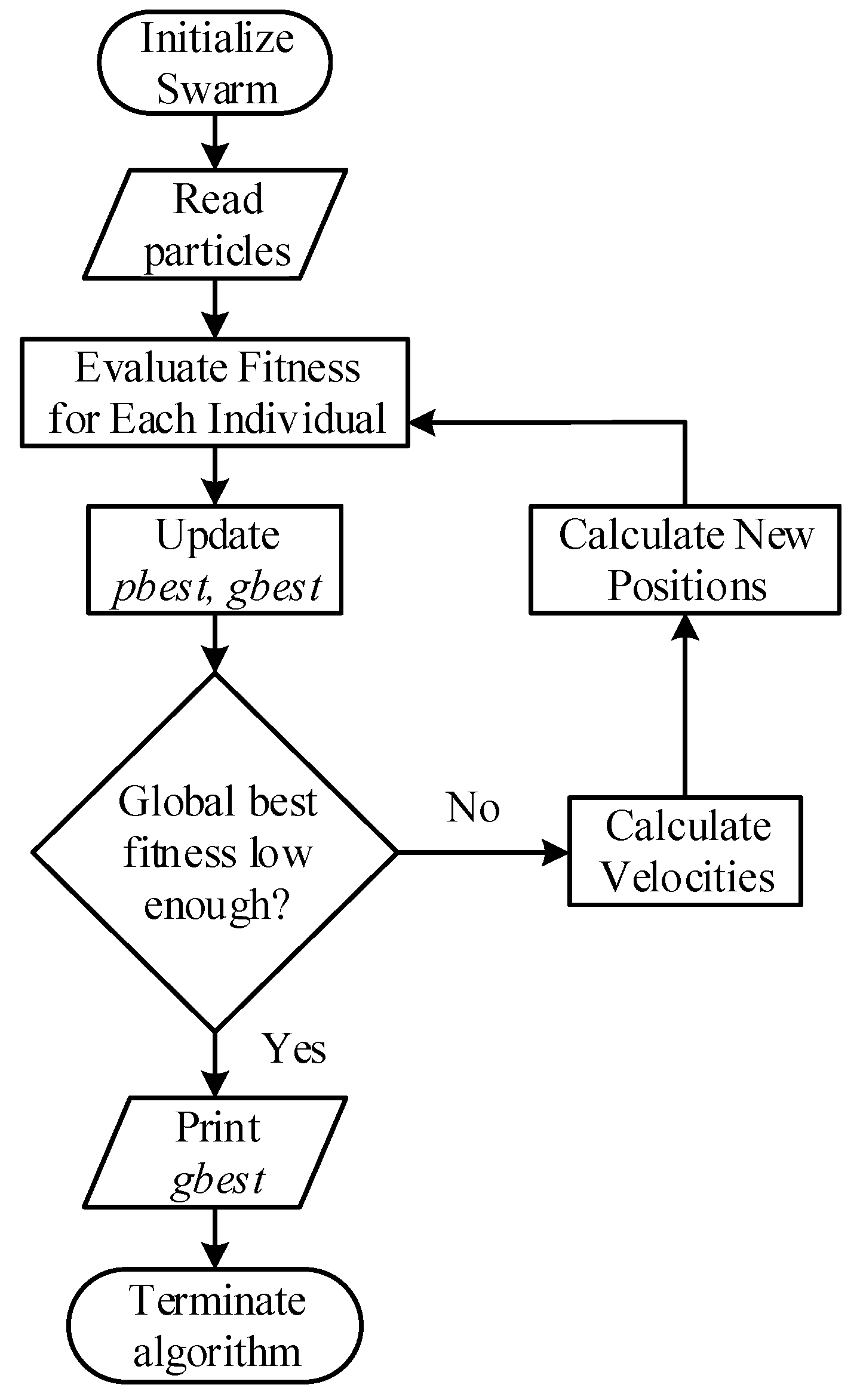
Figure 4 shows the basic flowchart of the PSO algorithm. Whenever the global best fitness, f, reaches a value less than a prespecified limit, e.g., f = 1 × 10⁻⁹ in this application, the algorithm terminates for each PSO calculation window.

3.2. Determination of Cost Function

In this application, the TLN1 technique is chosen to eliminate the six lowest-order sidekick harmonics, given as the 5th, 7th, 11th, 13th, 17th, and 19th, in the output voltage waveform of the inverter since even-order harmonics are not present if an odd quarter-wave symmetric pattern is used, and all triplen harmonics are eliminated in the line-to-line voltages for a three-phase, three-wire system. This results in a switching frequency of 750 Hz. For this sample application, the equation set in (11) is to be solved.

A new set of equations given in (12) is obtained by rearranging equations in (11) and using the M expression given in (7). The cost function T_n, and the fitness value, f, of a SHEM angle set can be expressed by squaring the left hand sides of the equations in (12) and then summing them up as given in (13). In (13), γ should be set to a value higher than 10 to converge the solution more rapidly. Furthermore, T₁ in (12) has crucial importance in determining V_c and hence adjusting Q_s to the prespecified set value.

$$\begin{gathered} b_1=\frac{4}{\pi } \frac{V_{dc}}{2}\left[-1-2{\displaystyle \sum }_{k=1}^7{\left(-1\right)}^k\cos \left({\alpha }_k\right) \right]={\widehat{V}}_c \\ {b}_n=\frac{4}{n\pi } \frac{V_{dc}}{2}\left[-1-2{\displaystyle \sum }_{k=1}^7{\left(-1\right)}^k\cos \left(n{\alpha }_k\right) \right]=0 \end{gathered}$$

(11)

where, ${\widehat{V}}_c=\sqrt{2}{V}_c$ is the peak value of the fundamental line-to-neutral voltage at the inverter output, V_dc is the DC link voltage, b_n is the peak value of the nth harmonic component (n = 5, 7, 11, 13, 17, and 19) as given in (2), and α_k is the SHEM angle to be determined for k = 1, 2, …, 7.

$$\begin{gathered} T_1=-1-\left[2{\displaystyle \sum }_{k=1}^7{\left(-1\right)}^k\cos \left({\alpha }_k\right)\right]-M=0 \\ {T}_n=-1-\left[2{\displaystyle \sum }_{k=1}^7{\left(-1\right)}^k\cos \left(n{\alpha }_k\right)\right]=0 \end{gathered}$$

(12)

$$f=\mu (\gamma T_1^2+T_5^2+T_7^2+T_{11}^2+T_{13}^2+T_{17}^2+T_{19}^2)$$

(13)

where γ and µ are the penalty values, respectively, for M and the angle constraint in (14).

$$0<{\alpha }_1<{\alpha }_2<{\alpha }_3<{\alpha }_4<{\alpha }_5<{\alpha }_6<{\alpha }_7<\frac{\pi }{2}$$

(14)

µ can be set to 10 for this sample application in order to eliminate invalid SHEM angle sequences rapidly during the on-line application of SHEM.

3.3. Results of the PSO Algorithm

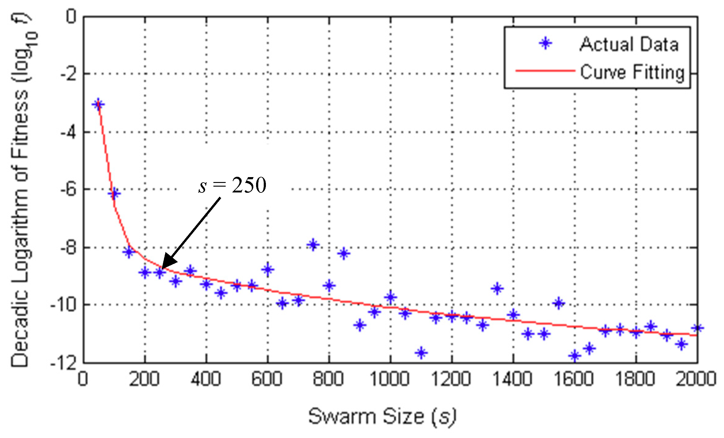
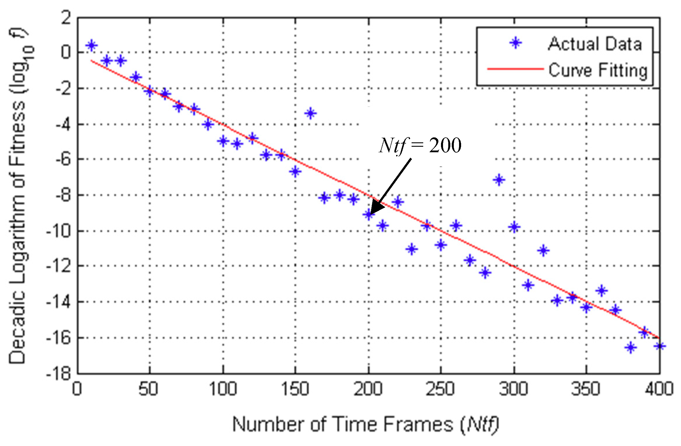
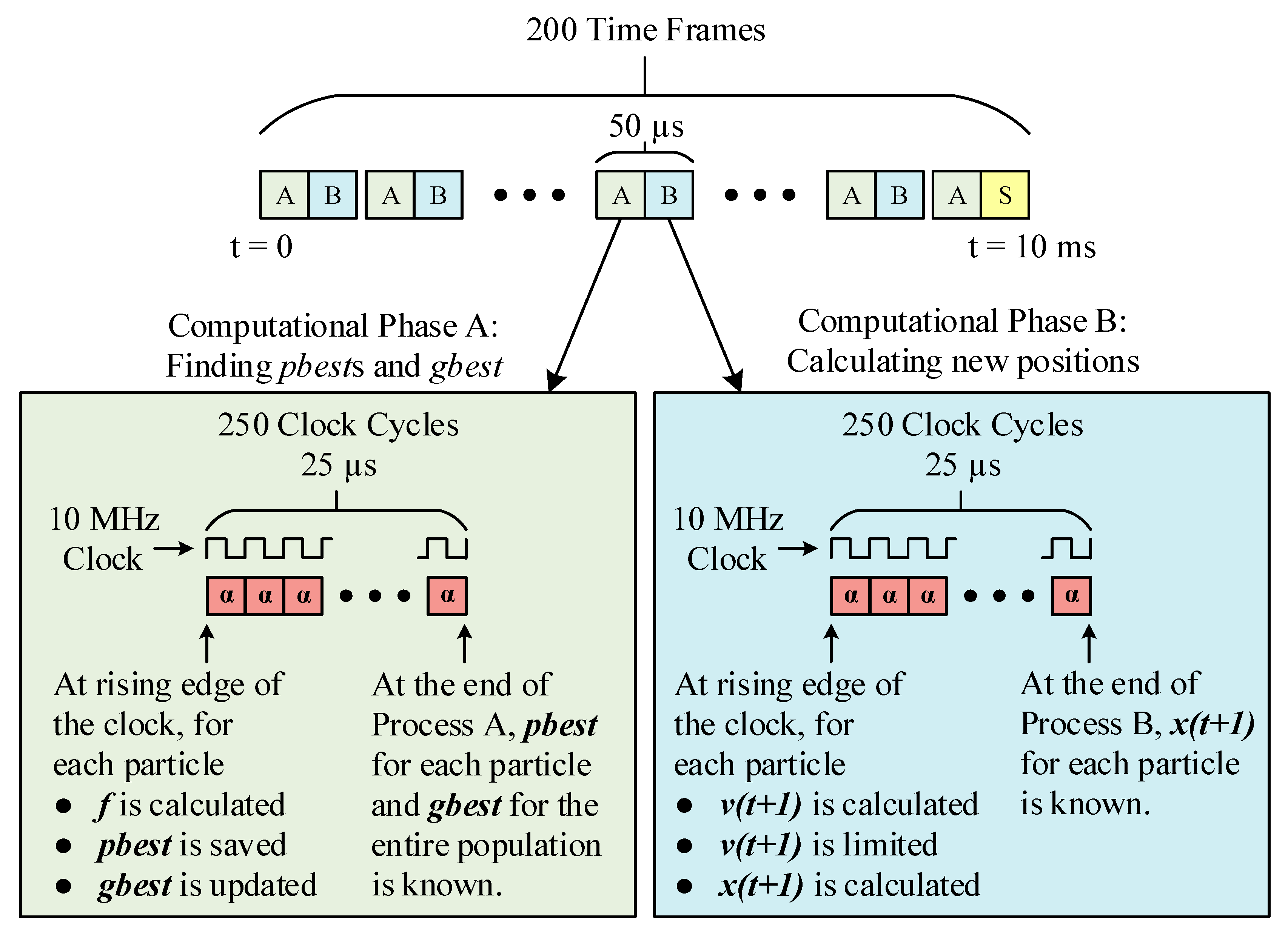
The parameters used in the PSO algorithm are first optimized in the MATLAB environment. Among these, the most important parameters affecting how fast the PSO algorithm converges are the swarm size, s, and the number of time frames, Ntf. The variations in fitness value, f against s, and Ntf are given in Figure 5 and Figure 6, respectively. The ideal value of f is zero. From Figure 5 and Figure 6, the optimum swarm size and number of time frames are chosen to be s = 250 and Ntf = 200, which correspond to a decadic logarithmic error, i.e., log₁₀ f = −9. The optimized and default values of all parameters used in the PSO algorithm are as given in

Table 2. Optimized Parameters of PSO Algorithm (optimized parameters are marked by *, and others are default parameters).

Symbol	Parameter	Value
β	Inertia weight	1
$c_1$	Cognition factor	2.8
$c_2$	Social factor	1.3
K	Constriction factor	0.729
s	Swarm size *	250
Ntf	Number of time frames *	200
γ	Modulation index penalty *	100
µ	Angle constraint penalty *	10

. SHEM angles from α₁ to α₇ are found against M by running the PSO algorithm in the MATLAB environment with optimized parameters in Table 2.

Random initialization of the PSO algorithm at time t = 0 (at start-up) can be made by utilizing the constraints defined for the problem by equating the initial value of M and hence the fundamental component of inverter’s output voltage to zero. Randomly chosen initial values usually cause convergence of the solution to a local minimum, especially for large numbers of SHEM angles, N. When the problem is generalized to eliminate all odd-order power system harmonics up to the 50th according to IEEE Std. 519-2014 [39] and IEC 61000-4-30 [40], the initial values of N number of SHEM angles can be distributed in the range of either,

• Case (I) from 0 to ξ = 90°, or
• Case (II) from 0 to ξ = 60°,

with respect to the zero crossing point on the rising edge of the fundamental line-to-neutral voltage waveform. Initial values of N number of SHEM angles can therefore be determined from the first equation in (12) by setting M to zero as given in (15).

$$M=-1+2\cos ({\alpha }_1)-2\cos ({\alpha }_2)+2\cos ({\alpha }_3)-2\cos ({\alpha }_4)+\dots +2\cos ({\alpha }_{N-2})-2\cos ({\alpha }_{N-1})+2\cos ({\alpha }_N)=0$$

(15)

In case (I), the SHEM angles are distributed between 0 and 90°, where the first SHEM angle α₁ is set to zero, and the last angle α_N to 90°. The angles from α₂ to α_N−1 are distributed to p sections, where p = (N + 1)/2, so as to eliminate pairwise the remaining cosine terms in (15). For N = 7, in the case study, α₁ = 0, α₂ = α₃ = 15°, α₄ = 60°, α₅ = α₆ = 75°, and α₇ = 90°. In order to cancel out the first term (−1) in (15), α₄ is set to 60°. 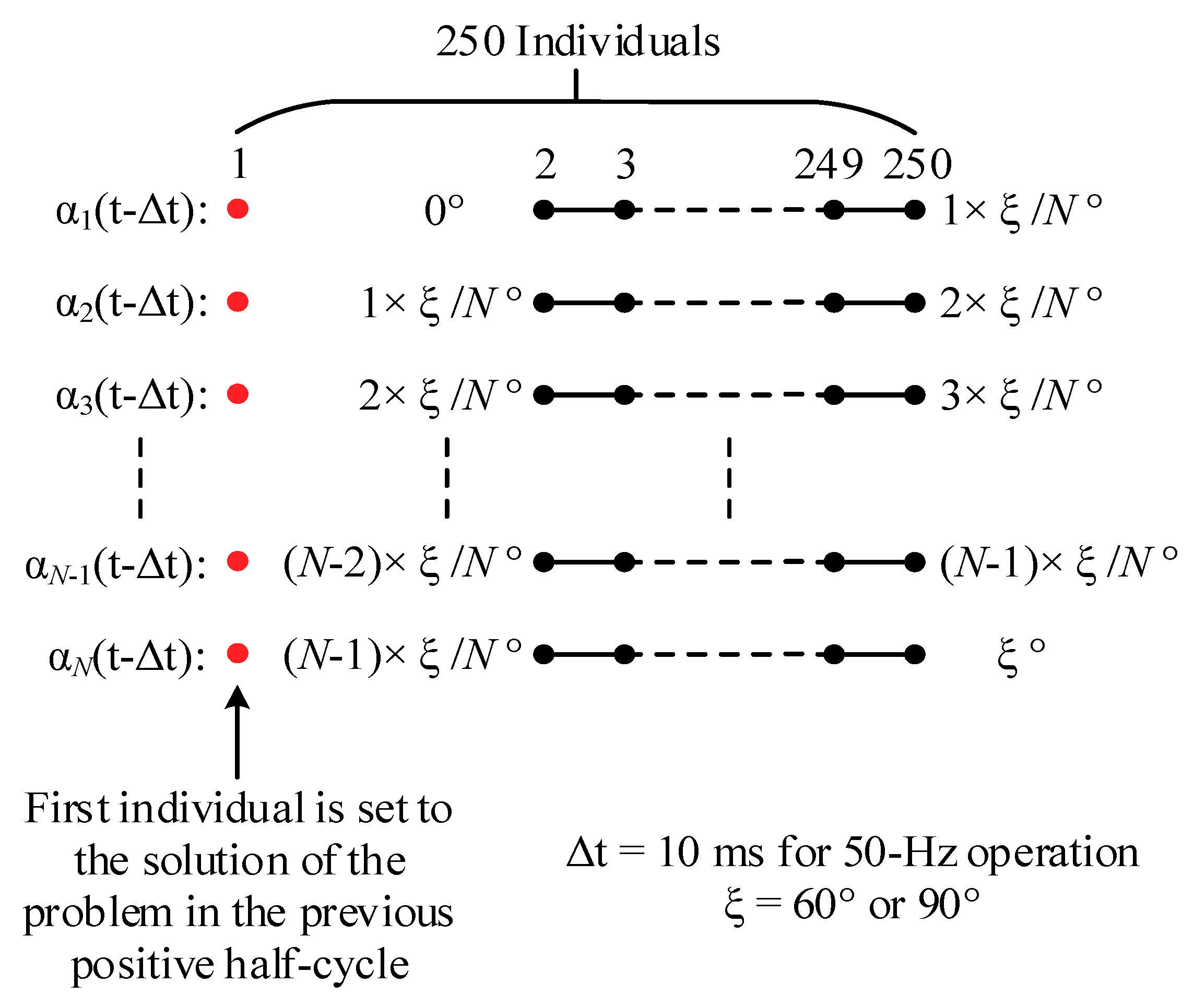Although the initialization procedure with M = 0 for case (I) which distributes SHEM angles over the quarter wave from 0 to 90° gives quite accurate results on the PSO algorithm for a low number of harmonics to be eliminated (for N = 3, 5, 7, and 9), this is not true for N > 9. However, in case (II), the SHEM angles are distributed between 0 and 60°, i.e., the last SHEM angle should be set to 60°, thus canceling the first term in (15). On the other hand, angles α₁ to α_N-1 are evenly distributed to p = (N + 1)/2 sections so as to cancel pairwise the remaining cosine terms. The generalization procedure for initial values of SHEM angles for case (II) is summarized in

Table 3. Generalized initialization procedure for SHEM angle sets. (N can be chosen to be any value among 3, 5, 7, …, 17; N = 17 eliminates all odd-order characteristic power system harmonics up to the 50th).

Initial Values of SHEM Angles, α1, …, αN to give M = 0
α1	α2	α3	α4	αk	αN−2	αN−1	αN
$\frac{60}{p}$	$\frac{60}{p}$	$\frac{60}{p}\times 2$	$\frac{60}{p}\times 2$	…	$\frac{60}{p}\times (p-1)$	$\frac{60}{p}\times (p-1)$	60°

. The initialization procedure in case (II) is simpler and more general than that of case (I).

There may be more than one solution for SHEM angles for any number N between 3 and 17. As an example, for N = 7, the optimum values of SHEM angles (α₁, α₂, … α₇) and the corresponding fitness values as a function of M are obtained by distributing the initial values in the range from 0 to 90° (case (I)) as given in

Table 4. SHEM Angles Found by the PSO Algorithm for N = 7 and Case I. (Yellow M: Not recommended, Red M: Impractical).

M	SHEM Angles, Degree							f
	α1	α2	α3	α4	α5	α6	α7
0.10	0.48	14.51	14.92	60.83	74.18	75.77	89.28	2.19 × 10−5
0.20	1.23	14.69	15.54	61.66	73.42	76.62	88.57	4.37 × 10−7
0.30	1.86	14.56	15.81	62.49	72.63	77.44	87.87	4.02 × 10−8
0.40	2.52	14.49	16.12	63.33	71.86	78.27	87.18	8.43 × 10−9
0.50	3.19	14.48	16.47	64.19	71.10	79.13	86.51	4.42 × 10−9
0.60	3.87	14.51	16.83	65.07	70.37	80.04	85.89	2.51 × 10−9
0.70	4.56	14.58	17.20	66.01	69.69	81.03	85.35	2.44 × 10−9
0.80	5.25	14.70	17.59	67.15	69.20	82.26	85.06	4.74 × 10−9
0.90	5.92	14.88	17.99	69.88	70.35	84.64	85.89	7.50 × 10−5
0.95	5.94	14.89	17.93	69.24	69.25	88.77	89.27	3.03 × 10−2

. However,

Table 5. SHEM Angles Found by PSO Algorithm for N = 7 and Case II. (Yellow M: Not recommended, Red M: Impractical).

M	SHEM Angles, Degree							f
	α1	α2	α3	α4	α5	α6	α7
0.10	14.14	15.31	29.14	30.57	44.15	45.76	59.16	2.23 × 10−5
0.20	13.33	15.68	28.26	31.14	43.24	46.47	58.33	4.94 × 10−7
0.30	12.48	16.01	27.35	31.69	42.33	47.19	57.48	8.22 × 10−8
0.40	11.61	16.32	26.41	32.22	41.38	47.92	56.61	1.12 × 10−8
0.50	10.72	16.59	25.42	32.71	40.39	48.62	55.71	5.52 × 10−9
0.60	9.80	16.80	24.37	33.13	39.31	49.31	54.78	5.06 × 10−9
0.70	8.84	16.90	23.21	33.41	38.09	49.92	53.76	3.22 × 10−9
0.80	7.81	16.77	21.83	33.33	36.53	50.33	52.50	7.14 × 10−9
0.90	6.56	15.87	19.68	31.60	33.37	48.11	48.63	8.41 × 10−5
0.95	5.92	14.74	17.79	29.10	30.10	49.09	49.10	2.78 × 10−2

shows the optimum values of SHEM angles and fitness values for the same problem when the initial values of those angles are chosen according to the generalized procedure in Table 3 (case (II)). As can be understood from Table 4 and Table 5, the optimum values of SHEM angles are different for the same problem owing to the use of different initial values. Since the f values are very low, both solutions can be considered to be the global optimum points found by the PSO algorithm.

Much lower f values could be obtained by using time frames higher than 200 (Table 2) at the expense of a longer execution time. In this research work, the results given in Table 4 are used in the implementation.

The control range of M is divided into three subregions:

(a)

Impractical M values in which the difference between any two consecutive SHEM angles is less than 0.1°. The associated M values and the critical angles are marked by red color boxes in Table 4 and Table 5. As an example, the typical turn-off times for 1700 V 300 A SiC power MOSFET and HV IGBT are nearly 0.27 μs and 1.8 μs, respectively. Deadbands of 0.5 μs and 3 μs can be chosen in the implementation for these power semiconductors. These values for deadbands correspond to ~0.01° and ~0.06° for 50-Hz grid applications, respectively. In higher power applications, IGCT (alternatively ETO) requires a nearly 10-µs deadband, which corresponds to ~0.2°. Therefore, operation at M ≥ 0.95 is impractical for all power semiconductors.

(b)

M ≤ 0.10 and 0.9 ≤ M < 0.95 values are not recommended for implementation especially for Si IGBTs, which are marked by yellow color circles in Table 4 and Table 5.

(c)

The remaining M control range in Table 4 and Table 5 defines safe operating M values.

In order to justify the usefulness of the PSO algorithm and the generalized initialization procedure in applying SHEM for the elimination of odd-order power system harmonics up to the 50th, optimum SHEM angles have been found for N = 7, 9, 11, 13, 15, and 17, and sample results corresponding to M = 0.7 are given in

Table 6. SHEM Angles for N = 7, 9, 11, 13, 15, and 17, and M = 0.7 Optimized by PSO Usıng the Generalized Initialization Procedure in Table 3.

N	SHEM Angles for M = 0.7, Degree																	f
	α1	α2	α3	α4	α5	α6	α7	α8	α9	α10	α11	α12	α13	α14	α15	α16	α17
7	8.84	16.90	23.21	33.41	38.09	49.92	53.76	-	-	-	-	-	-	-	-	-	-	3.22 × 10−9
9	7.15	13.24	18.70	26.20	30.45	39.15	42.56	52.10	55.08	-	-	-	-	-	-	-	-	8.24 × 10−9
11	5.99	10.88	15.67	21.56	25.44	32.20	35.38	42.85	45.54	53.50	55.94	-	-	-	-	-	-	7.50 × 10−9
13	5.17	9.23	13.49	18.31	21.86	27.35	30.33	36.39	38.92	45.44	47.66	54.47	56.54	-	-	-	-	9.30 × 10−9
15	4.54	8.01	11.85	15.91	19.18	23.77	26.56	31.62	34.03	39.48	41.59	47.35	49.24	55.20	56.99	-	-	4.89 × 10−9
17	4.04	7.08	10.56	14.06	17.09	21.02	23.65	27.96	30.25	34.91	36.93	41.86	43.66	48.81	50.47	55.75	57.34	7.77 × 10−9

. The results of these analyses show that the PSO algorithm can be successfully used in an on-line application of SHEM provided that powerful computing hardware is available for each case.

4. On-Line Application of SHEM to a Small-Scale PV Supply

SHEM is applied on-line by PSO to a laboratory prototype of a small-scale PV supply consisting of a two-level, three-phase, and grid-connected IGBT inverter with variable DC link voltage. It performs direct power conversion to the AC grid, and is equipped with a FPGA-based digital control system. If the PV inverter were connected to the PV array via a boost-type DC-DC converter, a DC link voltage control strategy could be adopted for reducing the TDD in grid-connected PV inverters as recommended in [41].

4.1. Description of the Laboratory Prototype

The circuit diagram of the power stage and block diagram of the prototype’s FPGA-based controller is given in Figure 7. An IGBT module (SKiiP 12AC12T4V1), a DC link capacitor, and an FPGA board are mounted on a common printed circuit board (PCB). The controller features are (a) elimination of selected harmonics (5th, 7th, 11th, 13th, 17th, and 19th) in the output voltage waveforms of the voltage source inverter (VSI), (b) maximum power-point tracking, and (c) reactive power control. The PCB of the laboratory prototype, the grid connection of the PV inverter through an LCL filter, and the flat-roof mounted thin-film PV arrays are shown in Figure 8.

In order to implement the worst operating condition in the laboratory, i.e., a step change in V_dc from 600 V to 900 V, the power stage is supplied from a solar simulator (Chroma 62150H-1000S) and Q_set in Figure 7 is set to zero for unity power factor operation. However, for steady-state operation, the power stage is supplied from the thin-film PV array shown in Figure 8c.

4.2. FPGA Implementation of On-Line SHEM

In order to apply the on-line SHEM to the grid-connected, two-level, three-phase VSI, powerful computing hardware having very fast computational capability, a parallel operation ability, and a sufficient number of input/output (I/O) ports is required. In the sample application, all calculation steps of the seven SHEM angles by the PSO algorithm and the necessary control actions should be completed in a time period of less than a complete cycle (20 ms for a 50-Hz application). The numbers of digital inputs to the computing hardware and outputs which will be applied to the gate driver circuits of the power stage are, respectively, 8 and 6 as shown in Figure 7. The timing diagram in Figure 9 summarizes the operational principles of the sample system in Figure 7, including all control actions and on-line application of SHEM. All of these functions are performed by only one common FPGA board. The phase-locked loop (PLL) modules of all phases run for each 20-μs period. The instantaneous reactive power, Q_inv, is calculated in each 20-μs period to update M. The PSO module is running in synchronism with the phase A supply line-to-neutral voltage waveform to calculate SHEM angles in every positive half-cycle of v_an. New SHEM angles for the power semiconductors of the inverter circuit are then updated only once in the next full-cycles of the v_cn, v_an, and v_bn voltage waveforms successively in order to avoid generation of DC and even-order voltage harmonics. On the other hand, the MPPT algorithm runs continuously to update δ every second.

In this research work, an XEM6010-LX150 USB-2.0-integrated FPGA module from Opal Kelly is chosen in the implementation which satisfies the requirements mentioned above [42]. This module consists of a Xilinx Spartan-6 XC6SLX150-2FGG484 FPGA to perform all control actions of the VSI together with an analog-to-digital converter (ADC) μchip (ADC128S102) [43].

The implementation of the on-line SHEM was realized by utilizing a fixed-point library in the very high level design language (VHDL) code. The developed software is composed of two parts, one of which performs calculations sequentially, while the other carries out parallel operations. VHDL code runs at a 10 MHz system clock frequency, while the RAM blocks should run at a maximum 30 MHz clock frequency in order to be able to follow the operations in one clock period. The flow of the PSO algorithm is as illustrated in Figure 10. In this research work, it is aimed at determining SHEM angles α₁ to α₇ in a time period less than or equal to 10 ms. For this purpose, the 10 ms time period is divided into 200 time frames. Each time frame can be considered as an iteration in two steps, A and B. Therefore, each iteration will take 50 µs of time. In the first phase, A, in Figure 10 of each iteration, (12)–(14) are solved in a consecutive manner for 250 individuals, whereas for each individual the same equations are solved simultaneously. Each iteration in phase A utilizes values for SHEM angles obtained in phase B in the previous iteration as being their initial values.

At the end of phase A of each iteration, the pbest values in (8) for 250 individuals and the gbest value in (8) for the population are calculated. As can be seen from the velocity update Equation (8), the algorithm uses two random numbers between 0 and 1 for random searching of particles in the search space. For this reason, random number generation has been employed in the VHDL code by using a pseudo random number generator (PRNG) [44].

A linear feedback shift register (LFSR) is a PRNG using sequential shift registers to produce binary random numbers in a certain periodic sequence, whose period can be increased by using more registers. Therefore, a more random sequence with respect to the frame of the algorithm can be acquired [45]. A 12-bit LFSR was used for this purpose in the code. In phase B of the same iteration, the velocity in (8) and new positions in (9), i.e., new α₁ to α₇, are calculated for each individual consecutively. The new positions for 250 individuals will then be applied to the phase A of the next iteration as the initial values. In phase A of the last iteration step, the 200th iteration, 250 SHEM angle sets, one for each individual, are obtained and among these the one having the lowest fitness value (gbest) is chosen as the solution of the problem in phase S of the 200th time frame in Figure 10. These are the updated SHEM angles (e.g., those calculated in the green-colored PSO module box in Figure 9) that will be applied to gate driver circuits of the power stage in the next full-cycles of the v_cn, v_an, and v_bn voltages as illustrated by green-colored arrows in Figure 9.

In the next positive half-cycle of the line-to-neutral voltage v_an (e.g., the violet-colored PSO module box in Figure 9), the PSO algorithm starts to run afresh regardless of whether the value of M remains the same or not. The PSO algorithm is initialized according to the lattice diagram given in Figure 11. Note that this diagram is a generalized one to cover all possibilities for N from 3 to 17. The first individual is the swarm leader, which tends to guide other individuals towards the solution. To initialize the PSO algorithm in the new positive half-cycle, the first individual utilizes the final values of the SHEM angles α₁ to α_N calculated in the previous positive half-cycle as the initial values of α₁ to α_N.

Only the initial value vectors corresponding to the 2nd and 250th individuals are marked on Figure 11, while the others are evenly distributed according to the lattice structure. The maximum SHEM angle ξ can be chosen as either 60° or 90°. In the prototype system, N = 7 and ξ = 90° were used. The performance of the FPGA implementation of on-line SHEM is verified in the following subsection experimentally by applying a step variation to M from 0.1 to 0.9.

4.3. Hardware Co-Simulation Results

The FPGA program written in VHDL code is run in real-time to determine the system clock frequency limits and to verify the correct operation of primarily the PSO submodule and secondarily the PLL, DC link voltage controller, and reactive power calculation submodules via Opal Kelly’s FrontPanel interface. In order to observe the performance of the on-line application of SHEM, a step change is given to M from 0.1 to 0.9 in the PSO module and the resulting responses of the SHEM angles α₁ to α₇ are recorded by using a digital storage oscilloscope (DSO) through digital-to-analog converters (DACs). The step change in M from 0.1 to 0.9 corresponds to a variation in V_dc much wider than 900 to 600 V. This is because M would vary in the range from 0.5 to 0.9 for a V_dc variation range from 900 V to 600 V in the field application.

The responses of the PSO module against the step change in M are as given in Figure 12 in both the transient-state and the steady-state. The 10-ms window, which corresponds to a half-cycle of 50 Hz grid voltage, is marked by a blue-colored pulse. Steady-state values of SHEM angles read on the DSO screen for M = 0.1 and 0.9 are also marked by purple-colored pulses on the records given in Figure 12. These records show that on-line calculation of SHEM angles by the PSO algorithm works rapidly and successfully, and in nearly 5 ms of time the SHEM angles α₁ to α₇ reach their final values even for a drastic step variation of M from 0.1 to 0.9.

In the hardware co-simulation test, the SHEM angles determined by the PSO module are also captured from Opal Kelly’s FrontPanel interface for different values of M in the range from 0.1 to 0.9 as given in

Table 7. SHEM Angles Found by Hardware Co-simulation.

M	α1(°)	α2(°)	α3(°)	α4(°)	α5(°)	α6(°)	α7(°)	f
0.10	0.541	14.606	15.018	60.805	74.234	75.794	89.289	1.216 × 10−5
0.20	1.217	14.677	15.524	61.637	73.439	76.619	88.583	2.384 × 10−7
0.30	1.864	14.583	15.838	62.481	72.649	77.441	87.868	1.192 × 10−6
0.40	2.544	14.522	16.188	63.347	71.843	78.293	87.170	2.408 × 10−5
0.50	3.154	14.612	16.429	64.168	71.110	79.115	86.521	1.860 × 10−5
0.60	3.843	14.510	16.816	65.048	70.391	80.003	85.916	7.153 × 10−7
0.70	4.555	14.590	17.219	66.012	69.694	81.034	85.359	1.907 × 10−6
0.80	5.253	14.728	17.616	67.138	69.186	82.275	85.053	1.907 × 10−6
0.90	5.895	14.865	17.923	70.053	70.572	84.427	85.767	2.489 × 10−4

. It is worth noting that the SHEM angles in Table 7 are more accurate than the corresponding DSO readings. That is the main reason why the steady-state values of SHEM angles for M = 0.1 and 0.9 in Figure 12 are slightly different from the corresponding values in Table 7. Fitness values of SHEM angle calculations against M variations are given in the last column of Table 7.

In the implemented system, higher f values have been obtained in comparison with the target fitness value of f = 1 × 10⁻⁹ in Figure 5 and Figure 6. This is attributed to the fact that the random number generator in the FPGA module is implemented to produce 12-bit random numbers and SHEM angles are realized as 24-bit fixed-point logic vectors. Twenty-four-bit random number generation and 32-bit fixed-point logic vector usage would give much lower f values. Nevertheless, when the SHEM angles calculated by the FPGA and corresponding to the worst case fitness value of 2.489 × 10⁻⁴ in Table 7 are applied to the MATLAB model of the PV supply, the individual low-order 5th, 7th, 11th, 13th, 17th, and 19th harmonic contents of the output line-to-line voltage waveform are found to be less than 0.5% with respect to the fundamental value. Thus, the fitness values in Table 7 are found to be quite acceptable in this application.

4.4. Limitations of Computing Hardware in On-line Application of SHEM

In this research work, on-line application of SHEM is implemented by using a XEM6010-LX150 USB-2.0-integrated FPGA module containing a Xilinx Spartan-6 XC6SLX150-2FGG484 FPGA to calculate seven SHEM angles continuously.

Table 8. Utilization report of FPGA Used in the Experimental System to Calculate Seven SHEM Angles in Real-Time.

Slice Logic Utilization	Available Number	Used		Utilization
		PSO Code	Total Code	PSO Code	Total Code
Slice Registers	184304	5080	9920	2%	5%
Slice LUTs	92152	8142	32794	8%	35%
Fully-Used LUT-FF Pairs	37683	2652	5031	7%	13%
Bonded IOBs	338	24	57	7%	16%
Block RAM/FIFO	268	84	104	31%	38%
BUFG/BUFGCTRL/BUFHCEs	16	2	3	12%	18%
DSP48A1s	180	105	177	58%	98%

shows the utilization report of the chosen FPGA while running only the PSO code and also the total code including all control and protection actions. As can be understood from the last row of Table 8, the chosen FPGA is working at its limit from the viewpoint of the number of DSP48A1 slices. Each DSP slice contains an 18-bit × 18-bit multiplier and a 48-bit accumulator to perform high-performance arithmetic and signal-processing actions.

One hundred and five DSP slices have been used to run the PSO code and 177 of the available 180 DSP slices have been used to run the total code in each half-cycle of the supply voltage waveform. It is obvious that in order to calculate a higher number of SHEM angles up to 17, high-performance computing is required. This can be achieved either by (a) using a much more powerful FPGA chip, which has much higher DSP slices, such as 740, 1920, and 3600, than the one used in the research work, (b) operating more than one moderately powerful FPGA for parallel computing, or (c) using a proper GPU together with a real-time operating system.

4.5. Field Test Results

The field performance of the real-time SHEM angle calculations by the PSO algorithm has been obtained on the prototype of a small-scale, grid-connected PV supply in Figure 8a with direct DC-to-AC conversion. Line-to-line voltage waveforms of the PV inverter and the corresponding harmonic voltage spectra are given in Figure 13 and Figure 14 when V_mpp = V_dc = 560 V and 667 V, respectively. These results show that the recommended method eliminates the target low-order harmonics (n ≤ 19) successfully. For elimination of all odd-order harmonics up to the 49th, 17 SHEM angles, instead of seven, are to be calculated on-line by using a PSO algorithm with higher computational complexity and more powerful digital computing hardware. This would increase the switching frequency from 750 Hz to 1750 Hz according to (1).

The 400-V line-to-line grid bus to which the prototype PV supply delivers power is slightly distorted (THD $\cong$ 1.8%) owing to the presence of the 3rd, 5th, and 7th harmonic voltage components. The line current waveform injected into the grid and its harmonic spectrum are as shown in Figure 15 when the PV supply delivers 800 VA to the grid at 0.8 p.f. lagging (the inverter is operating in its capacitive region). Although the TDD of the line current for the given test conditions is 4.1%, it contains some low-order harmonics, such as the 3rd, 5th, and 7th, which are not produced by the PV inverter, but sinked by the LCL filter tuned to 291 Hz and connected to the grid terminals. Harmonic current contributions of the PV inverter and the grid can be separated by using the method recommended in [46,47]. If the grid voltage waveform were a less distorted one, the TDD of the line current waveform would be much lower than 5%.

Since the reactive power delivered to the grid is determined by Q control loop and SHEM angles, and hence the magnitude of the fundamental component of the inverter’s output voltage, the performance of the resulting system is tested in the field for different Q_set values. Since in this application of instantaneous p-q theory only the average values of v_d, v_q, i_d, and i_q are taken into account, Q and Q_set are the actual and set values of the reactive power at 50-Hz supply frequency, respectively. Figure 16 shows the readings of an energy analyzer corresponding to Q_set = 0 and Q_set = 500 VAr. In these snapshots, the apparent power and active power readings include also harmonic effects, while the Q values are calculated only from the fundamental components. These results show the success of the PSO module, DC link voltage, and reactive power controller blocks.

5. Conclusions

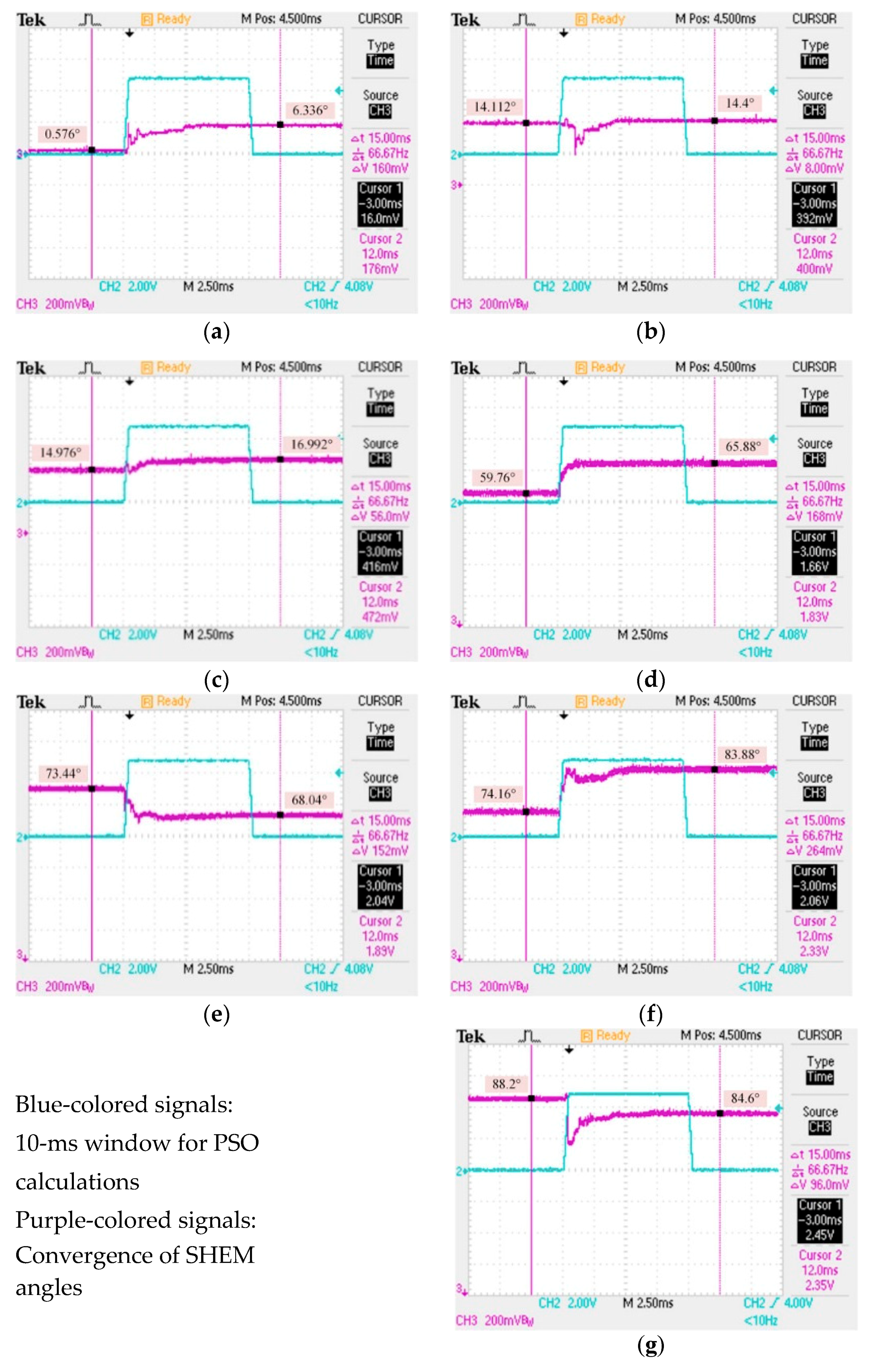
An off-line application of SHEM provides stepwise control of SHEM angles resulting in minimization of the selected harmonic components instead of their elimination. However, in the on-line application, switching angle sets can be continuously controlled by on-line calculation of SHEM angles, resulting in much better harmonic elimination performance and minimization of THDs. As reported in this paper for the first time, the six low, odd-order voltage harmonics of a grid-connected VSI with variable DC link voltage in a small-scale PV supply are eliminated on-line by using the developed PSO algorithm running on am FPGA controller successfully. The global best solution of the PSO algorithm is obtained with 250 individual particles, i.e., switching angle sets, within 200 time frames, resulting in a relatively small fitness value in the range from 10⁻⁷ to 10⁻⁴ depending on the modulation index, M. For a step change in M, all switching angles converge to the solution within a time period less than one half-cycle of the grid voltage, thus updating the switching instants of power semiconductors in every full-cycle of the output voltage.

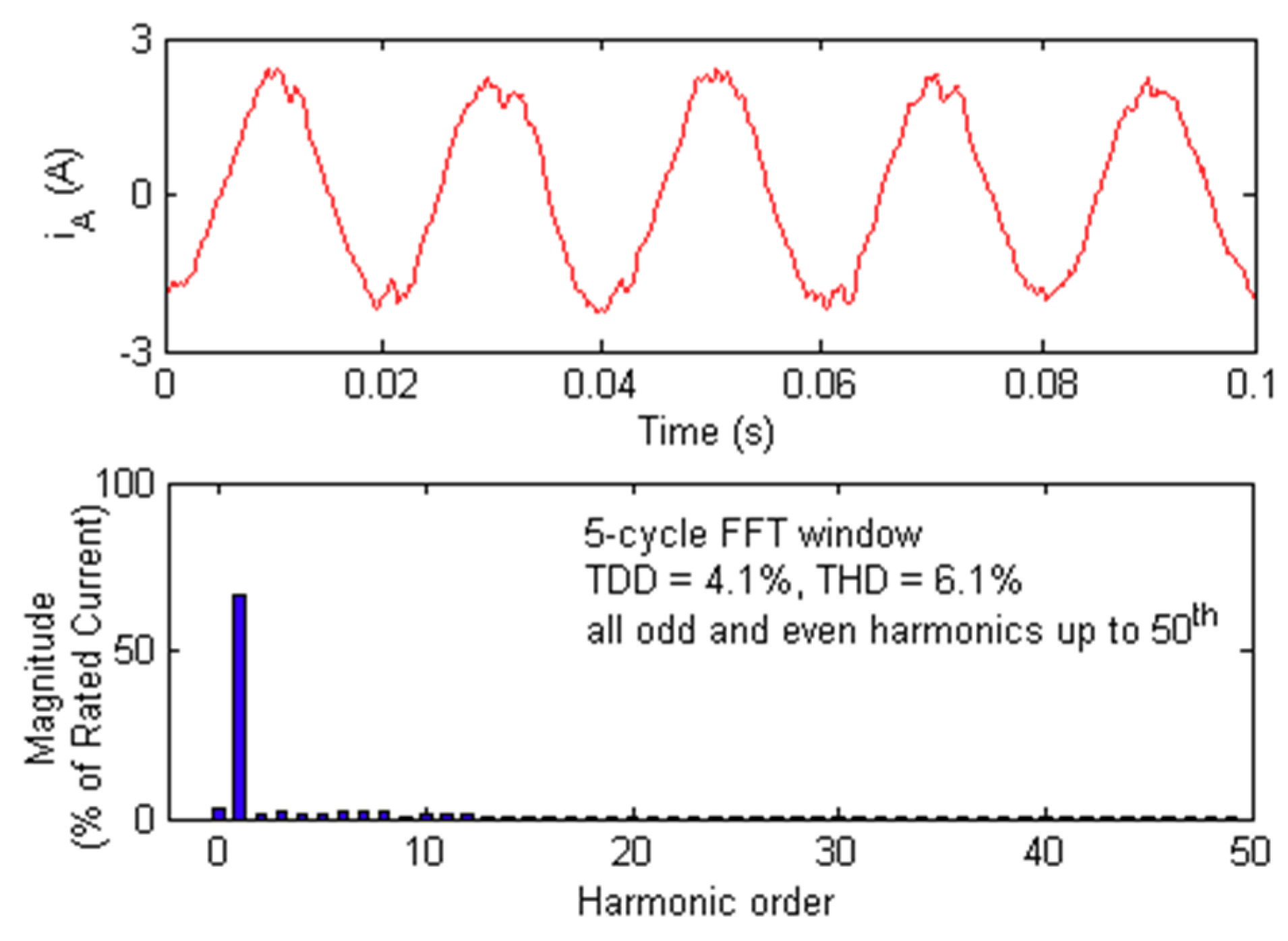
In order to eliminate all voltage harmonics up to the 50th continuously and rapidly, very powerful digital computing hardware is needed. This is an important requirement especially for variable frequency traction and industrial AC motor drives, where the motor drive is to be operated frequently at frequencies much higher than the rated frequency. In general, the maximum number of harmonics that can be eliminated or minimized in SHEM applications is dictated by the operational capabilities of power semiconductors employed in the VSC, such as the optimum switching frequency and turn-on and turn-off times. As an example, an SiC power MOSFET, as a wide-band-gap device permits the elimination of a number of harmonics much higher than that of IGBT-based VSCs in an on-line application of SHEM. Each recorded harmonic is the vectorial sum of the harmonic current component injected by the PV supply, and the associated one sinked by the LCL filter from the grid. Therefore, the harmonic current contribution of the prototype system can be assessed only by using a proper measurement and calculation method. On the other hand, the elimination of a much higher number of harmonics at the expense of a higher switching frequency would reduce significantly the size of the LCL filter and hence the amount of low-order harmonics sinked from the grid.