1. Introduction
Over the past few decades, trading algorithms have been improved in line with technological advancements and increasing accessibility of high-frequency data, i.e., transaction data recorded in very small successive intervals of time. Usage of such data is extremely beneficial to practitioners in establishing trading strategies and consequently achieving higher possible returns. For the same reason, new statistical and econometric tools for high-frequency data analysis have been developed, taking into account a number of distinct characteristic of these data, such as discreetness, unevenly spaced time intervals, long memory, market microstructure noise and price jumps. These properties have been comprehensively studied in the literature for better understanding the mechanism of the price formation as well as the variance of price returns [
1,
2,
3].
Estimation and forecasting of the variance of a financial time-series is still, and will remain for a long time, one of the major challenges for researchers and practitioners alike. Despite the enormous existing studies and various proposed approaches [
4,
5,
6], most of them do not deal with empirical high-frequency or intraday data for estimation of a true but unknown variance of returns, so-called integrated variance (IV), but use simulation data or just ignore some of their distinguishing properties. However, integrated variance can be efficiently estimated by the realized variance (RV) as the sum of equidistant intraday squared returns [
7]. It has been documented that realized variance converges in probability to integrated variance [
8]. Moreover, RV is a perfect measure of IV when intraday prices are observed continuously [
9]. On the contrary, when prices are exposed to a substantial amount of microstructure noise, the realized variance may not obtain consistency and asymptotic unbiasedness [
10,
11]. Common sources of market microstructure noise are discreteness of price observations, non-synchronous trading, bid–ask bounces, differences in trade sizes, etc. In real life, stock prices are only observed at discrete time points and high-frequency data are not available for all stocks and markets when trading is thin. RV is more contaminated with microstructure noise as sampling frequency increases, or in other words, when the time interval between successive observations declines [
12]. On the contrary, when sampling at a lower frequency, RV becomes less biased due to reduction of the noise [
13]. The widespread opinion is to sample sparsely from 5 min to 30 min, as suggested in the literature [
14]. On the other side, sparsely sampling reduces a significant amount of information, leading to inefficient RV estimation. For example, one might sample every 10 min from transactions data observed every second, which means that every 600th observation is selected. In that context, it is crucial to find an optimal sampling frequency for which the balance between efficiency and potential biasedness of the RV estimator is achieved [
14,
15]. The trade-off between sampling too frequently and sampling too rarely can be formalized by minimizing the root mean squared error of the estimator. A less formal approach of finding appropriate sampling frequency, but very popular in empirical work, is volatility signature plot [
16]. Nonetheless, the first consistent estimator of the IV proposed in the literature is a Two Times Scaled Realized Variance (TSRV). Estimator TSRV exhibits a nice asymptotic properties in the presence of the noise, while keeping all the data at the highest possible frequency. This is accomplished by taking a linear combination of the pre-averaged RV sampled at the two scales: fast time scale and low time scale [
15,
17]. However, when jumps occur, a two times scaled estimator becomes biased. Many jump robust estimators were established in the literature, but most of them are not robust to microstructure noise [
18,
19].
Additionally, a jump robust version of TSRV was proposed (RTSRV) [
20]. Both estimators, TSRV and RTSRV, respectively, are constructed to deal with highly liquid assets, e.g., observations sampled every few seconds. Otherwise, if sampling frequency is low to begin with, e.g., every minute, the bias of the estimator might be over-corrected. This is the main reason why this paper considers high-frequency data obtained exclusively from developed European stock exchanges. Therefore, the key objective of the paper is to provide empirical evidence of RTSRV superiority among realized volatility competitors, as the best approximation of IV. For the same reason, the jump robust two times scaled estimator is used as a benchmark in this research. Although, this research does not cover the most recent period of the historical data, obtained findings contribute to academics as well as market participants by indicating an optimal slow time scale frequency that should be used when RTSRV is applied for each analyzed market individually. There is no consensus in the literature on which estimator is better for which market. This research provides an answer to that question. Along with comparison of RTSRV as a benchmark realized volatility against other RV estimators, the purpose is to conclude which markets are more contaminated with the microstructure noise, and in which markets price jumps are more present. Thus, concrete findings offer valuable suggestions to users when employing high-frequency data in financial management. Once again, it should be noted that performance of RV estimators which are robust to microstructure noise, price jumps or both have been documented in previous studies based on simulation data or data from the US markets [
21,
22,
23], while there is no research that analyzes the developed European stock markets, as in this paper. Less developed markets are not considered due to the poor quality of high-frequency data which cannot be observed every second, while observations sampled at lower frequency are not welcome as the bias of the benchmark estimator might be over corrected. Moreover, the novelty of the paper is that it empirically demonstrates RTSRV robustness to both microstructure noise and price jumps, i.e., for each market under consideration of an optimal slow (low) sampling, frequency is determined to mitigate the sensitivity to microstructure noise without losing a significant part of intraday observations, while a threshold parameter is attentively selected for truncation purposes to mitigate the price jumps. In total, seven competing estimators are considered for comparison against benchmark volatility proxy of the IV. Pairwise comparison methods incorporate the Kolmogorov–Smirnov test on probability integral transformations, Mincer–Zarnowitz regression, and upper tail correlation from the Gumbel copula.
The rest of the manuscript is outlined as follows:
Section 2 presents the employed data and methods.
Section 3 provides empirical findings.
Section 4 offers discussion with respect to current results, while conclusions are provided in
Section 5.
2. Data and Methods
This study utilizes in total more than 195 million observations, over a 7-year period. Data of developed stock markets from 4 January 2010 to 28 April 2017 for Germany, Italy, France and UK were provided by Thomson Reuters Tick History (TRTH) service. Indices MIB, DAX, CAC and FTSE represent benchmarks from Italian, German, French and British stock exchanges. Despite the fact that historical data do not cover the most recent period, due to limited funding from the project which is completed four years ago, an extensive dataset exhibit representativeness with respect to the long period of time and the most liquid European stock markets which is strongly required for computation of proposed benchmark estimator RTSRV.
In
Table 1, the number of trading days and the number of 1-second observations are given. These numbers differ across observed European markets. The intraday data taken into consideration were during official trading hours from 9:00 a.m. until 5:30 p.m., five days a week.
Eight estimators of integrated variance, including a benchmark RTSRV, are presented in
Table 2. Each of them depends on sampling frequency
, i.e., the increment between two successive and equally spaced price observations
. The number of intraday returns
for every trading day is
. Since
, the lesser information is used when
increases. Moreover, realized variance
becomes unbiased when sampling frequency increases due to reduction of microstructure noise as a consequence of sparse sampling [
16]. However, the cost of sparse sampling is a high variance of an estimator (inconsistency) as a small number of observations is left for computational reasons. Not only does the microstructure noise contaminate realized variance, but also price jumps [
23,
24,
25]. Thus, a second estimator
is proposed in the literature as jumps robust estimator. The idea of [
7] who introduced a bipower variation, is that multiplication of
with the adjacent
will dampen the jump impact if it occurs even for sufficiently small
. Similar to bipower variation, two estimators also emerged in the literature, i.e., minimized and medianized realized variance
and
, respectively [
26]. According to [
21], both estimators follow a concept of the nearest neighbor truncation by the use of the minimum operator on blocks of two returns or median operator on blocks of three returns. They have better performance in the finite samples compared to bipower variation although
suffers from a similar exposure to zero returns as
.
A serious drawback of the aforementioned estimators is the lack of data when sampling sparsely. Opposite to that, Ref. [
27] proposed how to keep all the data but still have an unbiased and asymptotically consistent estimator of integrated variance. Thus, a two time scaled estimator
was introduced, which combines average subsampled realized variance at slow time scale
and realized variance
at fast time scale. In other words, when utilizing the two times scaled estimator, parameter
is the fast time scale, i.e., the highest possible sampling frequency available to the user, while the parameter
k is the slow time scale frequency which defines the number of subgrids. For practical reasons, it is common to keep the fast time scale fixed, while the slow time scale should be determined optimally by minimizing RMSE (root mean square error) of the estimator.
As previously highlighted,
is robust to microstructure noise as well as
and
, depending on the parameters
and
k, while
,
and
are robust to price jumps only. Robust versions of IV have also been designed in the presence of both jumps and noise. In particular, robust version of two times scaled realized variance
was designed by [
20]. This estimator requires one additional parameter
which is employed as a threshold with respect to indicator function
. The threshold
is usually set to 9 indicating if returns are larger than three standard deviations from the mean. If returns are larger than three standard deviations from the mean, the indicator function has value 0 and 1 otherwise. The last estimator which is considered in this paper for comparison is
designed by [
28]. This estimator can be understood as a threshold realized variance which uses jump detection rule
to truncate the effect of jumps. It has to be mentioned that all estimators are sensitive to the selection of sampling frequency, and criteria for optimal frequency should be considered. Comprehensive study with respect to these criteria can be found in [
13,
15].
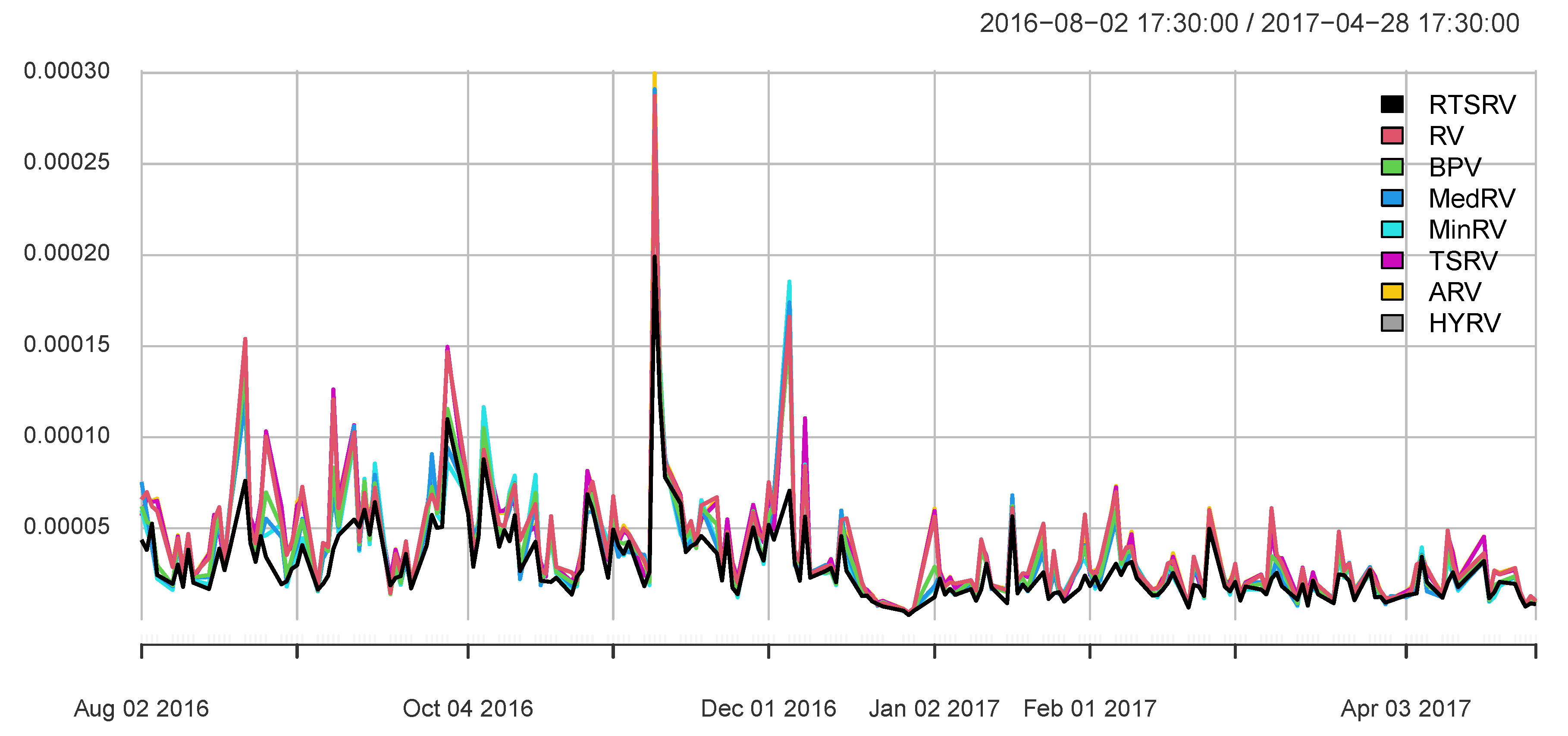
For better visual inspection of the differences between realized volatility measures, their performances are compared in
Figure 1, considering DAX index (Frankfurt Stock Exchange) within the selected range of data from 1 March 2017 until 31 March 2017.
After the computation of realized volatility measures with respect to optimal sampling frequency, three comparison methods are conducted in order to determine which volatility estimator fits the most to
as a benchmark. These three comparison methods are Mincer–Zarnowitz regression, probability integral transformation (PIT) test, and Gumbel copula upper tail dependence. Mincer–Zarnowitz regression is based on the overall performance of the realized volatility estimators. The PIT test was performed as a density goodness of fit procedure in order to test how the examined realized volatility estimators preform in comparison to
. The upper tail dependence was used because it examines what happens in the extreme values or tails. The
is defined as a benchmark because it is robust to market microstructure noise as well as price jumps and non-synchronous trading in the intraday stock price series, while other estimators do not possess these features. These advantages were found in a simulation study only [
20], but there is no strong empirical evidence of superiority of
considering developed European stock markets.
3. Empirical Results
Each comparison method is comprised of fitting seven realized volatility estimators to the benchmark . Before pairwise comparison, fixed parameters and are set in advance, as previously argued and , while the optimal slow time scale sampling frequency k was selected for each European market based on minimizing the RMSE of the benchmark.
3.1. Sampling Frequency Selection
The fast time scale sampling frequency
second is determined in front, according to data availability of the observed financial markets within the shortest, nonempty and equidistant intervals. In order to define the optimal slow time scale sampling frequency
k, the root mean square error (RMSE) of the benchmark
is used. The RMSE of the benchmark for each stock index was calculated as the sum of its squared bias and its variance, and afterwards the RMSE was minimized with respect to slow time scale frequency
k, which corresponds to the optimal number of non-overlapping subsamples or subgrids, over which the slow time scales sum of squared returns is averaged [
29].
Namely, it is suggested to use returns that are sampled as often as possible because one can get the maximum amount of information from data. However, if the sampling frequency is as high as it can be, it leads to a bias problem due to microstructure noise. There is a trade-off between the bias and efficiency while determining an optimal sampling frequency. One must establish the optimal sampling frequency for an observed financial market in order to reduce the bias but still keep the efficiency of the benchmark estimator. In the presence of jumps, there will also be bias in practical applications. Thus, it will have an effect on sampling frequency, which is also influenced by market structure, liquidity and microstructure noise. The way to increase the efficiency of estimators is to sub-sample (taking the average of an estimator across all possible sub-samples).
Even the robustness of the
to the choice of
k has been theoretically demonstrated by [
30], it is found at which optimal slow frequency a benchmark should be computed for each of four developed European markets (
Table 3).
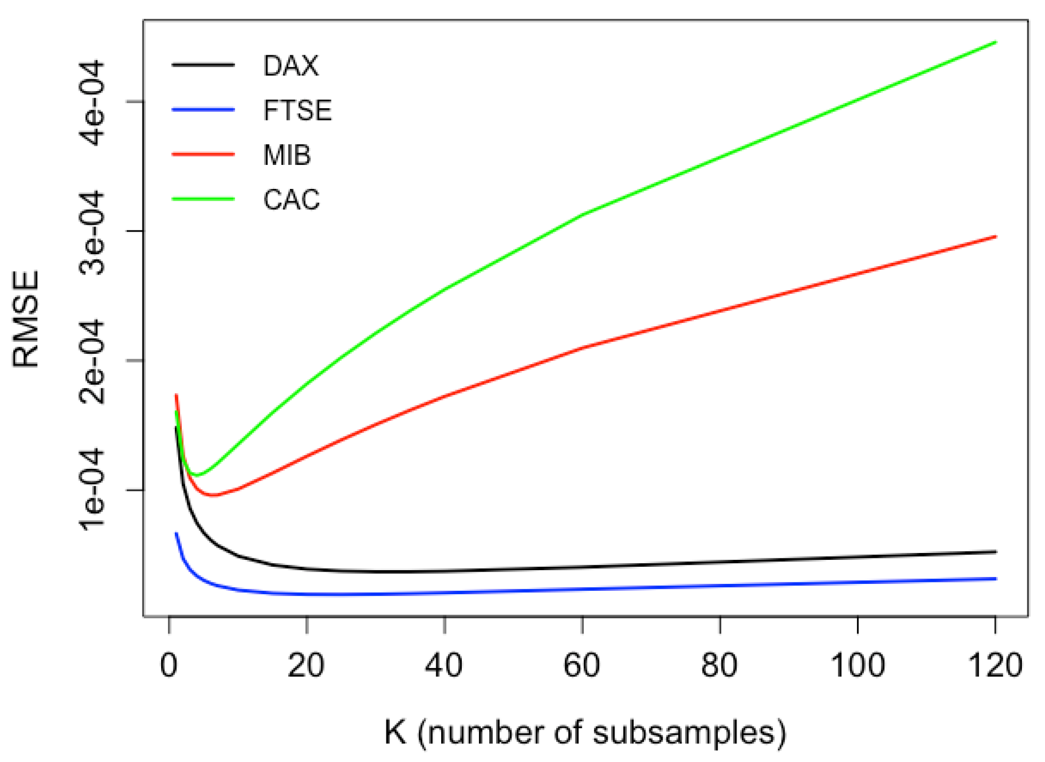
As can be seen in
Figure 2, the optimal sampling frequency for Germany is 20 s; for the UK, it is 30 s; for Italy, it is 13 s; and, for France, it is 10 s.
Figure 2 shows the root mean squared error (RMSE) of the robust two times scaled estimator for each stock market index against the number of subsamples.
3.2. Mincer–Zarnowitz Regression
After finding an optimal slow frequency,
can be easily computed for each developed market, so that the effect of microstructure noise becomes attenuated. Consecutively, the Mincer–Zarnowitz regression was estimated using GLS rather than OLS to improve the power and the size of the test on how well the realized volatility competitor
fits to the benchmark:
The Minzer–Zarnowitz regression approach is of great benefit for discriminating between competing estimators because it examines the bias [
31,
32]. In particular, it was jointly tested two restrictions on the parameters within a single null hypothesis
and
. The results, including
statistics and estimated parameters, are presented in
Table 4.
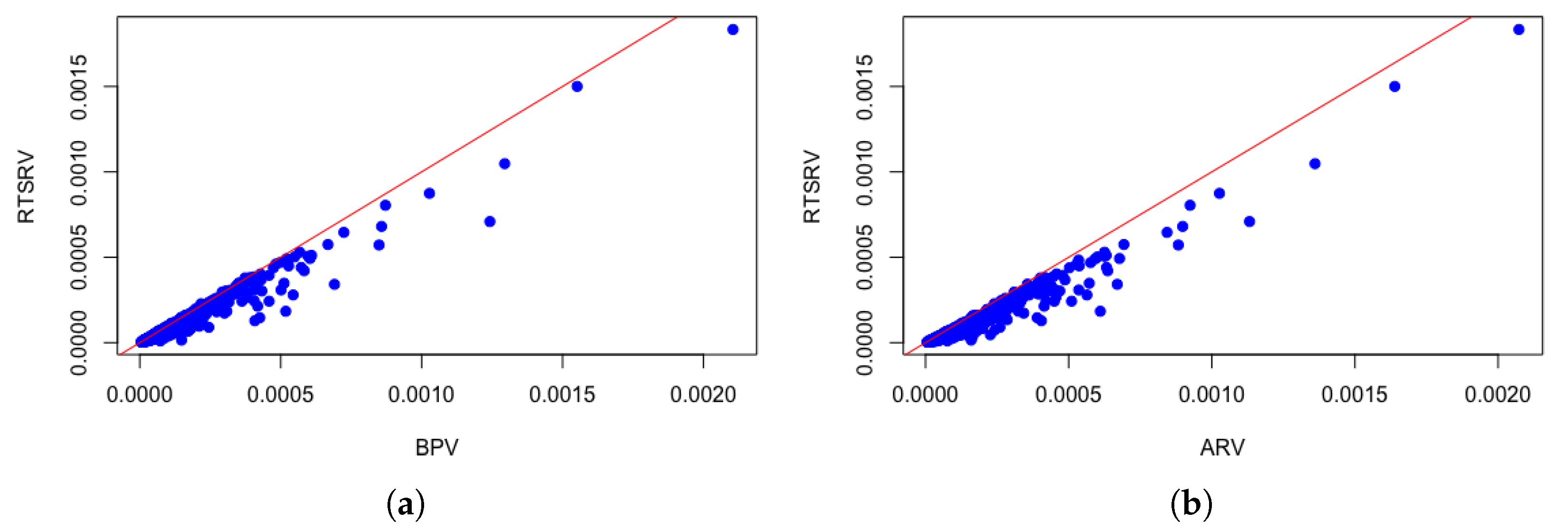
For all four European markets under consideration and seven volatility estimators, the null hypothesis was rejected at a significance level of 1%. This showed how seven observed volatility estimators do not fit well to the benchmark. For illustration purposes,
Figure 3a,b are scatter plots indicating that both bipower variation
, which is jump robust only, and average subsampled realized variance
, which is only robust to microstructure noise, underestimate the benchmark.
3.3. Probability Integral Transformation and Kolmogorov–Smirnov Test
The probability integral transformation (PIT) was used to check whether the difference between and other competing volatility estimators is uniformly distributed. Namely, uniform transformed volatility estimates are obtained by empirical distribution function of the same estimates from the given estimator. The pairwise differences between two uniform transformed estimates are used as an input in testing the null hypothesis about uniform distribution of these differences by the Kolmogorov–Smirnov test.
The results, including Kolmogorov–Smirnov test statistics, are presented in
Table 5. For all European markets, the null hypothesis was rejected at a significance level of 1%, indicating a significant divergent performance of each competing estimator towards a benchmark.
3.4. Upper Tail Dependence
This research utilizes the upper tail dependence coefficient, a result of the Gumbel copula function, which is found useful for measuring extreme dependence, i.e., a dependence above a high quartile. While the Mincer–Zarnowitz regression and Kolmogorov–Smirnov test have not demonstrated the preference of a specific estimator, the copula-based approach can be a powerful and suitable for comparison [
29]. The paper focuses on a Gumbel copula as an extreme value copula that is not elliptical, due to the similar behavior of volatility estimator over time, and sometimes takes on extremely large values. The Gumbel copula function is given by:
where
are in fact PIT transformations computed as an empirical cumulative distribution function, with parameter
that controls the upper tail dependence accordingly
. A Gumbel copula is fitted to each pair of volatility estimators of which one is always
, and Gumbel parameter is estimated using the pseudo likelihood method (PLM).
The results given in
Table 6 present the upper tail dependence coefficient
based on estimated
from the Gumbel copula function. The results indicate that, for Italy, Germany, and the UK,
has the highest upper tail dependence with
,
, and
volatility estimators.
4. Discussion
Each competing volatility estimator was tested against benchmark using Mincer–Zarnowitz regression, PIT test, and upper tail dependence measurements within the Gumbel copula. The results of the first two methods for comparison of the realized volatility estimators indicate that , , , and underestimate the performance of estimates during severe stress and price jumps. Therefore, the results do not give a clear answer regarding which estimator fits the best to the benchmark. In that case, the upper tail dependence is a favorable method to use because it takes into account extreme values.
Among all the competing estimators, only jump robust ones have produced almost similar volatility estimates as . In the case of France, is best fitted with , , , and volatility estimators. As is robust to microstructure noise, it is of no surprise that estimates are as good as .
While estimating the integrated variance in a simulation study, looking at the asymptotic properties, the two times scaled estimator was shown to be consistent and unbiased to microstructure noise [
33].
The results are important to financial analysts and investors because they offer a recommendation which realized the volatility estimator to use for the observed stock indices. This research contributes to the previous studies with an empirical dataset consisting of high-frequency price observations comprising four main European market indices (DAX, CAC, FTSE and MIB) because there are very few studies that take into account the calculations of realized volatility estimators on developed European markets.
5. Conclusions
The popularity of high-frequency data is enlarging, even if it is still hard to obtain such data. However, the scientific focus on research of volatility estimators has increased and expanded the knowledge from the already existing literature. This increase is mainly due to the availability of high-frequency data. Even though realized variance
is the most used high-frequency estimator, it is biased due to microstructure noise. The benchmark robust two times scaled realized variance
is microstructure noise and jump robust. In this research, the data observed are intraday 1 s observations. It is determined that the optimal sampling frequency for the robust two times scaled realized variance
is from 10 to 30 s. There is no consensus in the previous studies regarding the “best” realized volatility estimator. The objective of this research paper is to determine whether the robust two times scaled realized variance
is a superior volatility estimator for each of the four considered European markets by performance comparison of two groups of estimators, i.e., estimators which are robust to microstructure noise as well as jump-robust estimators. Due to inconclusive results from Mincer–Zarnowitz and PIT test, the upper tail dependence was introduced because it examines the events in tails i.e., extreme values. The results indicated that the medianized block of three returns
performed most similar to
for Italy, Germany and UK. For France, the two times scaled realized variance
realized volatility estimator was the most similar (approximately equal) to the benchmark. Since the medianized block of three returns
is robust only to price jumps, we conclude that the Italian, German and UK financial markets are more contaminated by price jumps than by microstructure noise. The French financial market is more contaminated by microstructure noise than by price jumps. This contributes to the existing literature in several ways. The main finding considers the selection of optimal slow time scale frequency in favor of two times scaled estimator in each market individually, at the same time ensuring robustness to price jumps. Another novelty is the usage of a combination of three tests for benchmarking: Mincer–Zarnowitz regression, PIT test and upper tail dependence test within the Gumbel copula where the results are given for each of the observed developed European markets. The direction of further research would be to investigate the realized covariance of different assets [
34,
35] using high–frequency data, which is a great challenge due to non–synchronization issue, presence of co–jumps and sampling frequency selection.


