1. Introduction
Despite years of research, our theoretical understanding of neural networks, their loss landscape and their behavior during training and testing is still limited. A recent novel theoretical analysis of neural networks, using quiver representation theory given by [
1], has been introduced, where the algebraic and combinatorial nature of neural networks is exposed. Among other things, the authors present a by-product of representing neural networks through the lens of quiver representation theory, i.e., the notion of
neural teleportation.
This is the mathematical foundation that explains why practitioners of deep learning have observed the property of scale invariance for the very particular case of neural networks with positive scale invariant activation functions, see, for example, the work of [
2]. Nevertheless, this type of invariance has not been studied or observed in its full generality, for example, across batch norm layers, residual connections, concatenation layers or activation functions other than ReLU. Even more, it has been claimed, for example, by [
3], that there is no scale invariance across residual connections. This is because it is not until a neural network is drawn as a quiver that the invariance of the network function under isomorphisms across any architecture becomes obvious (see
Appendix A for an illustration of this). Positive scale invariance also restricts the type of scaling factor, reducing them to positive real numbers and positive scale invariant activation functions, while neural teleportation allows to teleport any neural architecture with any non-zero scaling factor.
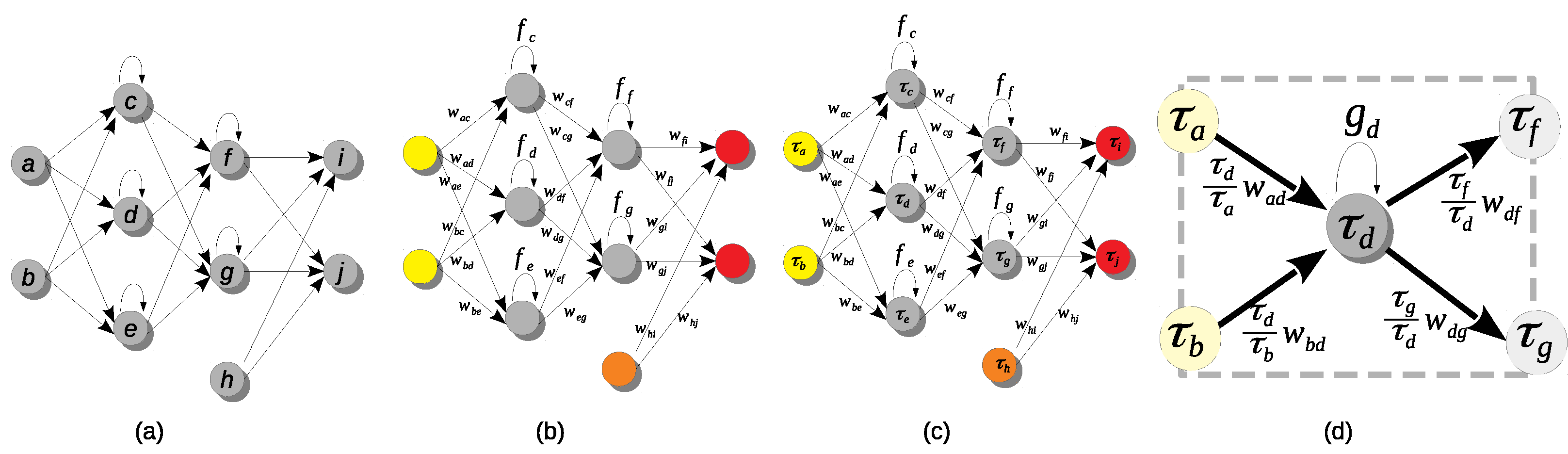
In this work, we intend to exhibit empirical evidence that using quiver representation theoretic concepts produces measurable changes on the behaviours of deep neural networks. Due to its mathematical nature, neural teleportation is an intrinsic property of every neural network, and so it is independent of the architecture, the activation functions and even the task at hand or the data. Here, we perform extensive experiments on classification tasks with feedforward neural networks with different activation functions and scaling factor sampling.
As will be explained later, neural teleportation is the mathematical consequence of applying the concept of isomorphisms of quiver representations to neural networks. This process has the unique property of changing the weights and the activation functions of a network while, at the same time, preserving its function, i.e., a teleported network makes the same predictions for the same input values as the original, non-teleported network.
Isomorphisms of quiver representations have already been used on neural networks, often unbeknownst to the authors, through the concept of
positive scale invariance (also called
positive homogeneity) of some activation functions, see [
2,
3,
4,
5]. However, representation theory lays down the mathematical foundations of this phenomenon and explains why this has been observed only on networks with positive scale invariant activation functions. Following the quiver representation theoretic approach to neural networks, it becomes clear that any neural network can be teleported with an isomorphism, as opposed to what is remarked in the literature. Namely, it has been claimed that there is no scale invariance across residual connections [
3] or on the parameters beta and gamma for batch norm layers [
6]. We explain (see
Appendix A for illustrations on residual connections and batchnorm layers) how the quiver approach is essential to apply teleportation to any architecture.
The concept of positive scale invariance derives from the fact that one can choose a
positive number
c for each hidden neuron of a
ReLU network, multiply every incoming weight to that neuron by
c and divide every outgoing weight by
c and still have the same network function. Note that models such as maxout networks [
7], leaky rectifiers [
8] and deep linear networks [
9] are also positive scale-invariant. This concept in previous works is always restricted to positive scale-invariant activation functions and to positive scaling factors. However, the generality in which quiver representation theory describes neural networks allows to teleport any architecture, with any activation function and any non-zero scaling factor.
In this paper, we show that neural teleportation is more than a trick, as it has concrete consequences on the loss landscape and the network optimization. We account for various theoretical and empirical consequences that teleportation has on neural networks.
Our findings can be summarized as follows:
Neural teleportation can be used to explore loss level curves;
Micro-teleportation vectors have the property of being perpendicular to back-propagated gradients computed with any kind and amount of labeled data, even random data with random labels;
Neural teleportation changes the flatness of the loss landscape;
The back-propagated gradients of a teleported network scale with respect to the scaling factor;
Randomly teleporting a network before training speeds up gradient descent (with and without momentum). Actually, we also found that one teleportation can accelerate training even when used at the middle of the training.
3. Previous Work
It was shown that positive scale invariance affects training by inducing symmetries on the weight space. As such, many methods have tried to take advantage of it, for example, [
2,
4,
11,
12]. Our notion of teleportation gives a different perspective as (i) it allows any non-zero real-value CoB to be used as scaling parameters, (ii) it acts on any kind of activation functions, and (iii) our approach does not impose any constraints on the structure of the network nor the data it processes. Moreover, neural teleportation does not require new update rules as it only has to be applied
once during training to produce an impact.
Refs. [
2,
3] accounted for the fact that ReLU networks can be represented by the values of “basis paths” connecting input neurons to output neurons. Ref. [
3] made clear that these paths are interdependent and proposed an optimization based on it. They designed a space that manages these dependencies, proposing an update rule for the values of the paths that are later converted back into network weights. Unfortunately, their method only works for neural nets having the same number of neurons in each hidden layer. Furthermore, they guarantee no invariance across residual connections. This is unlike neural teleportation, which works for any network architecture, including residual networks.
Scale-invariance in networks with batch normalization has been observed by [
6,
13], but not in the sense of quiver representations.
Positive scale invariance of ReLU networks has also been used to prove that common flatness measures can be manipulated by the re-scaling factors [
5]. Here, we experimentally show that the loss landscape changes when teleporting a network with positive or negative CoB, regardless of its architecture and activation functions. Note that the proofs of [
5] are for two layer neural networks while we teleport deeper and much more sophisticated architectures, and provide empirical evidence of how teleportation sharpens the local loss landscape.
4. Neural Teleportation and the Loss Landscape
Despite its apparent simplicity, neural teleportation has surprising consequences on the loss landscape. In this section, we underline such consequences and lay empirical evidence for it.
4.1. Inter- and Intra-Loss Landscape Teleportation
As mentioned before, teleporting a positive scale invariant activation function
with a positive
results in
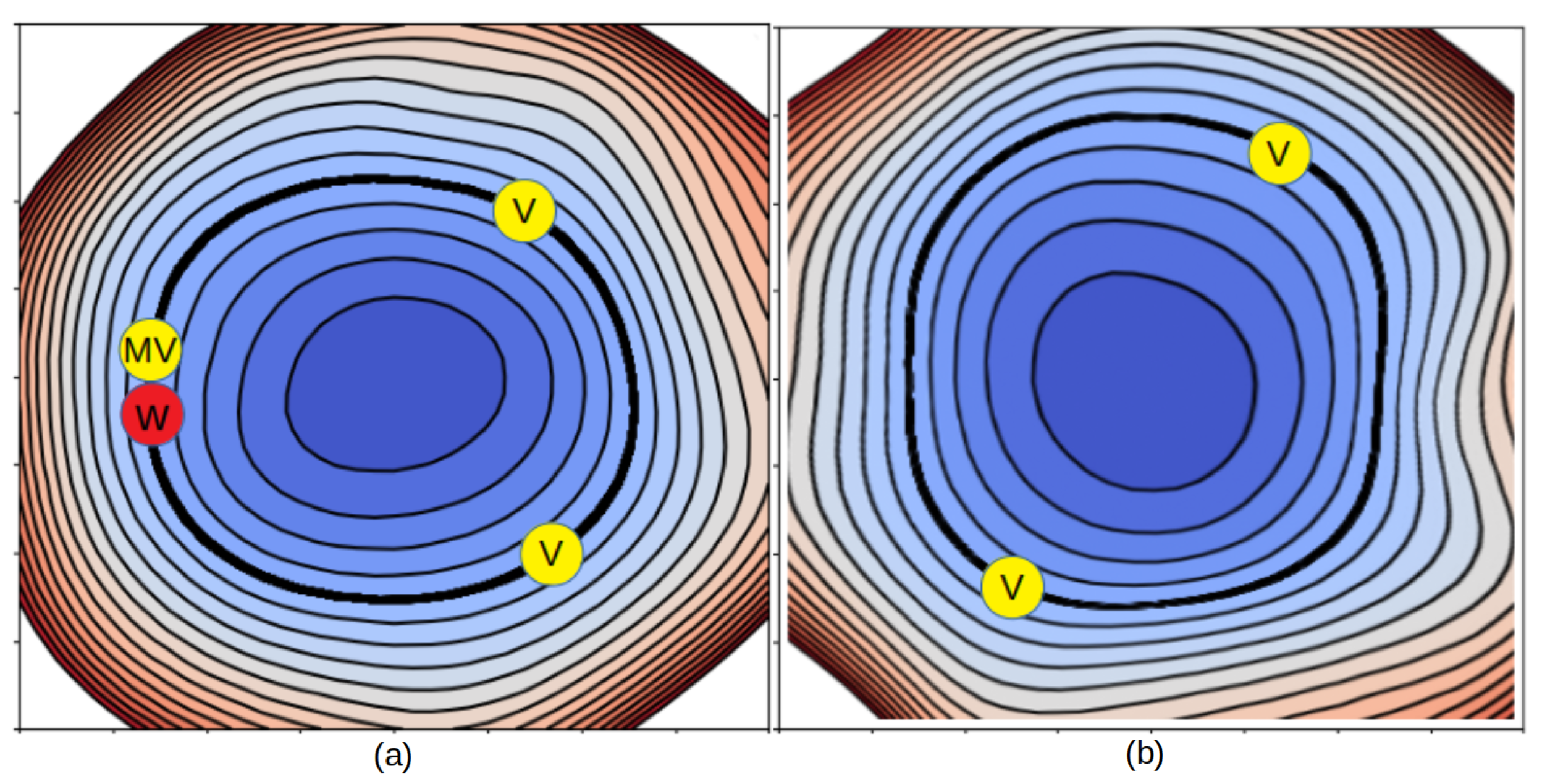
. This means that the teleported network ends up inside the same loss landscape but with weights
V at a different location than
W (c.f.,
Figure 2a). In other cases (for
negative or non-positive scale invariant activation functions
), neural teleportation changes the activation function and, thus, the overall loss landscape. For example, with
and
a ReLU function, the teleportation of
becomes:
.
Thus, the way CoB values are chosen has a concrete effect on how a network is teleported. A trivial case is when
for every hidden neuron
, which leads to no transformation at all:
and
. For our method, we choose the CoB values by randomly sampling either of two distributions. The first one is a uniform distribution centered on 1:
with
. We call
the
CoB-range; the larger
is, the more different the teleported network weights
V will be from
W. In addition, when this sampling operation is combined with positive scale invariant activation function (like ReLU), the teleported activation functions stay unchanged (
) and, thus, the new weights
V are guaranteed to stay within the same landscape as the original set of weights
W (as in
Figure 2a). We, thus, call this operation an
intra-landscape neural teleportation.
The other distribution is a mixture of two equal-sized uniform distributions: one centered at
and the other at
:
With high probability, a network teleported with this sampling will end up in a new loss landscape, as illustrated in
Figure 2b. We, thus, call this operation an
inter-landscape neural teleportation.
4.2. Loss Level Curves
Since
can be assigned any non-zero real values, a network can be teleported an infinite amount of times to an infinite amount of locations within the same landscape or across different landscapes. This is illustrated in
Figure 2, where
W is teleported to 5.
We validated this assertion by teleporting an MLP 100 times with an inter-landscape sampling and a CoB-range of . While the mean average difference between the original weights W and the teleported weights V is of (a large value considering that the magnitude of W is of ), the average loss difference was in the order of , i.e., no more than a floating point error.
4.3. Micro Teleportation
One can easily see that the gradient of a function is always perpendicular to its local level curve (c.f. [
14] chap. 2). However, back-propagation computes noisy gradients that depend on the amount of data used, that is, the batch-size. Thus, the noisy back-propagated gradients do not a priori have to be strictly perpendicular to the local loss level curves.
This concern can be (partly) answered via the notion of
micro-teleportation, which derives from the previous subsection. Let us consider the
intra-landscape teleportation of a network with positive scale invariant activation functions (such as ReLU) with a CoB-range
close to zero. In that case,
for every neuron
and the teleported weights
V (computed following Equation (
1)) end up being very close to
W. We call this a
micro-teleportation and illustrate it in
Figure 1a (the MV dot illustrates the micro teleportation of W).
Because V and W are isomorphic, they both lie on the same loss level curve. Thus, if is small enough, the vector between W and V is locally co-linear to the local loss level curve. We call a micro-teleportation vector.
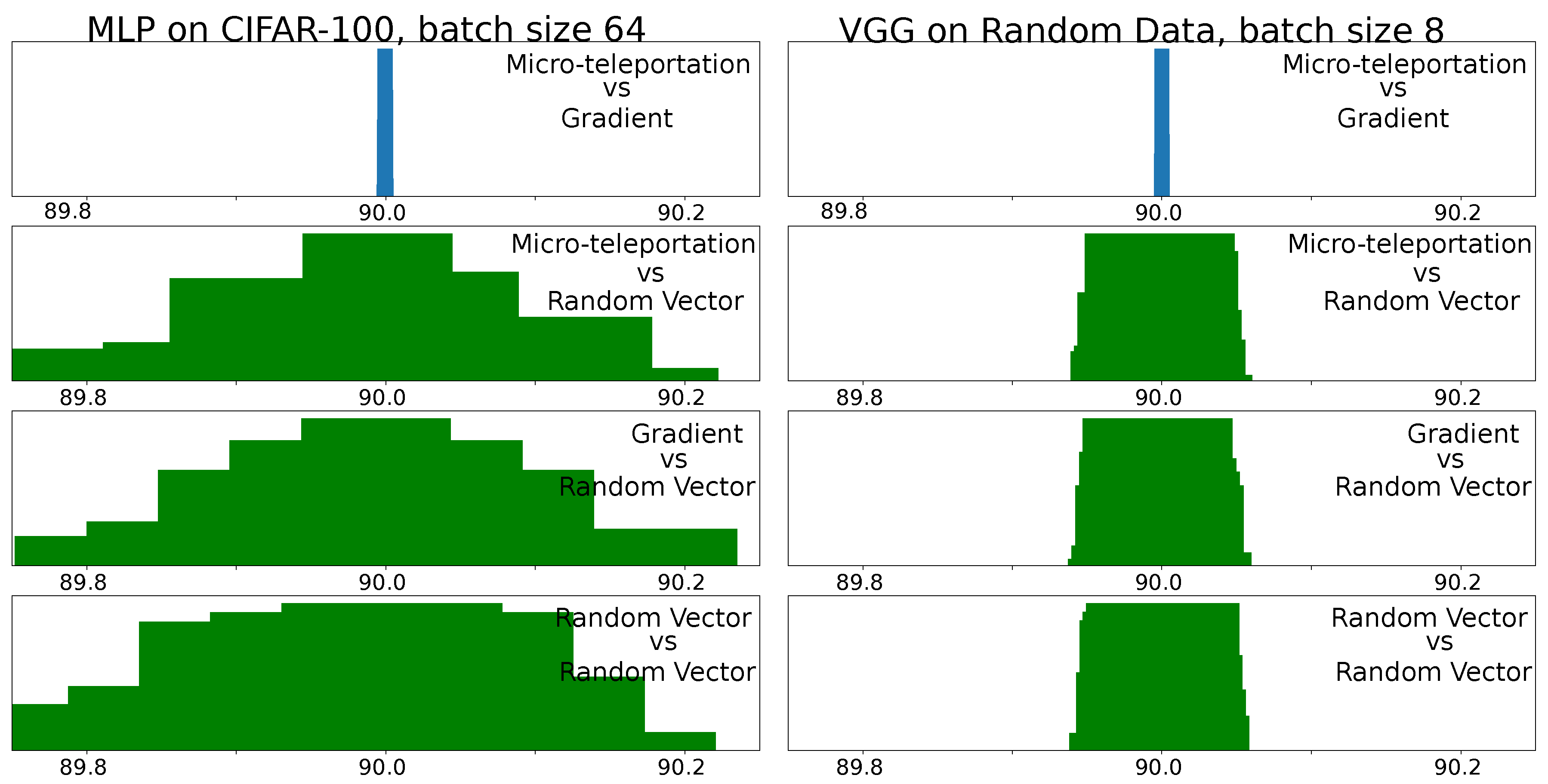
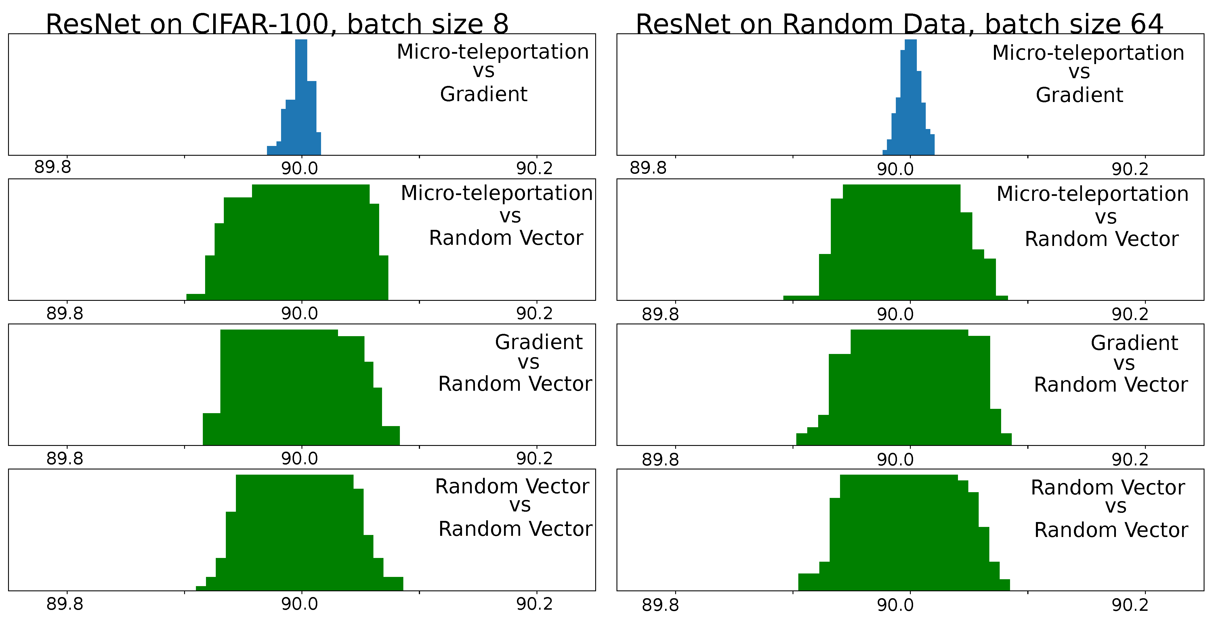
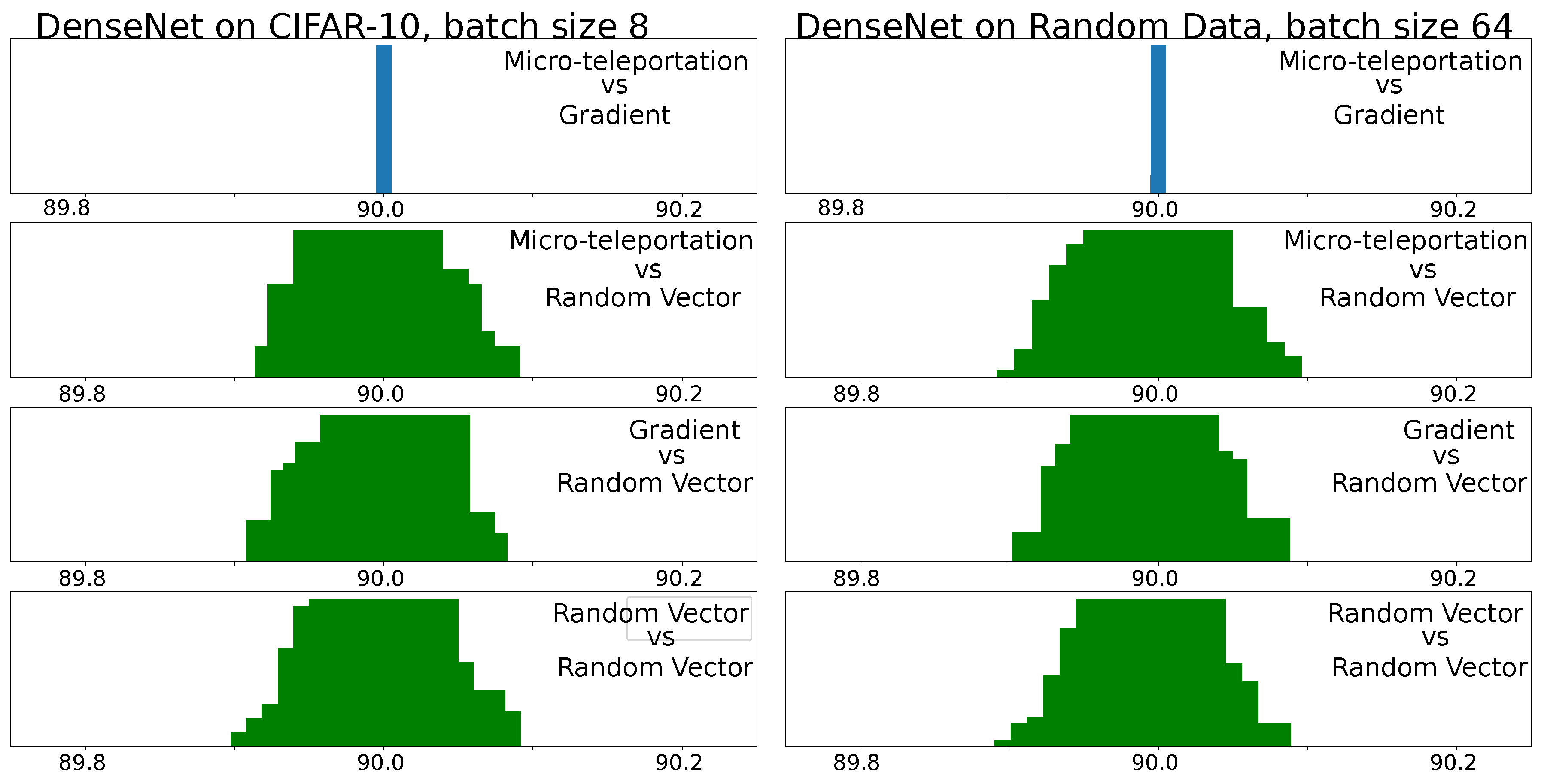
A rather counter-intuitive empirical property of micro-teleportations is that is perpendicular to any back-propagated gradient across different batch sizes, because we know that the back-propagated gradient depends on the batch size but the teleportation does not. Moreover, if one uses L2 regularization the loss is not the same anymore before and after teleportation, so it does not make sense that micro teleportation is perpendicular to the gradient as we were using L2 regularization in our experiments. This surprising observation leads to the following conjecture.
Conjecture 1: For any neural network, any dataset and any loss function, there exists a sufficiently small CoB-range σ so that every micro-teleportation produced with it is perpendicular to the back-propagated gradient with any batch size.
We empirically assessed this conjecture by computing the angle between micro-teleportation vectors and back-propagated gradients of four models (MLP, VGG, ResNet and DenseNet) on three datasets (CIFAR-10, CIFAR-100 and random data) 2 different batch sizes (8 and 64) with a CoB-range
. A cross-entropy loss was used for all models.
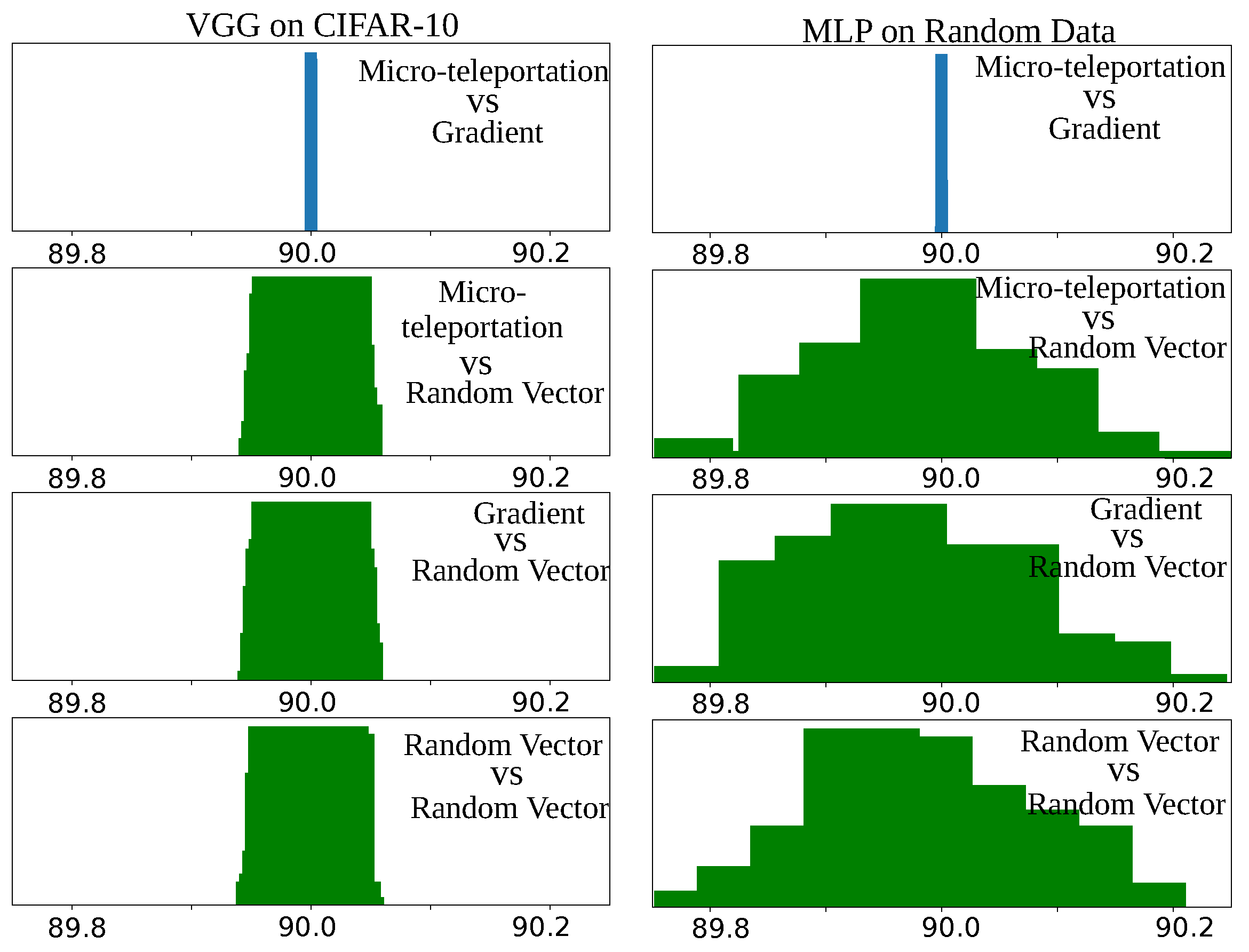
Figure 3 shows angular histograms for VGG on CIFAR-10 and an MLP (with one hidden layer of 128 neurons) on random data (results for other configurations are in the
Appendix A). The first row shows the angular histogram between micro-teleportation vectors and gradients. We used batch sizes of 8 for MLP and 64 for VGG. As can be seen, both histograms exhibit a clear Dirac delta on the
angle. As a mean of comparison, we report angular histograms between micro-teleportation vectors and random vectors, between back-propagated gradients and random vectors, and between random vectors. While random vectors in a high-dimensional space are known to be quasi-orthogonal (c.f work of [
15]), by no means are they exactly orthogonal, as shown by the green histograms. The Dirac delta of the first row versus the wider green distributions is a clear illustration of our conjecture.
These empirical findings suggest that although back-propagation computes noisy gradients, their orientation in the weight space does not entirely depend on the data nor the loss function. In other words, back-propagation computes gradients that point to directions perpendicular to micro-teleportation vectors, but micro-teleportation vectors do not depend on the loss nor the data. Finally, we note that this conjecture is false if one adds a regularization term that does not depend directly on the output of the network, for example, regularization adds a term that depends on the weights but not on the output of the network.
4.4. Teleportation and Landscape Flatness
It has been shown by [
5] for positive scale invariant activation functions, that one can find a CoB (called
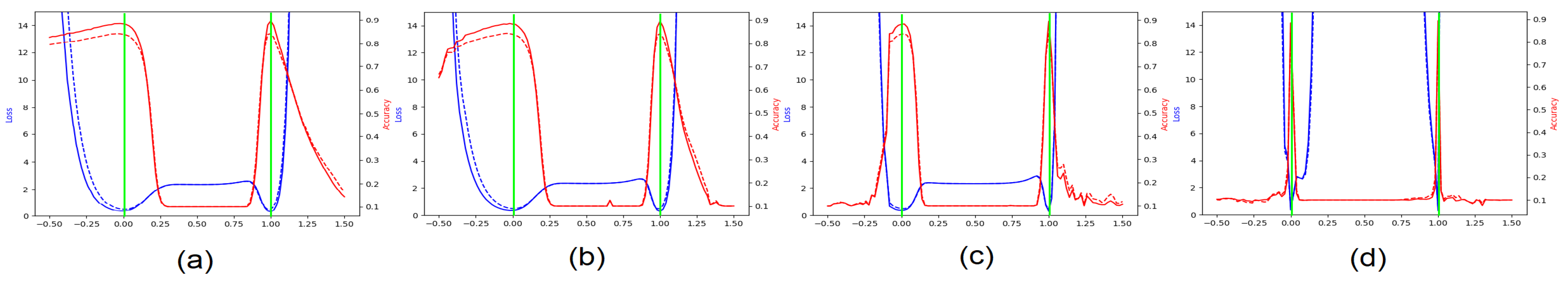
reparametrization in their paper) so that the most commonly used measures for flatness can be manipulated to obtain a sharper minimum with the exact same network function. We empirically show that neural teleportation systematically sharpens the found minima, independently of the architecture or the activation functions.
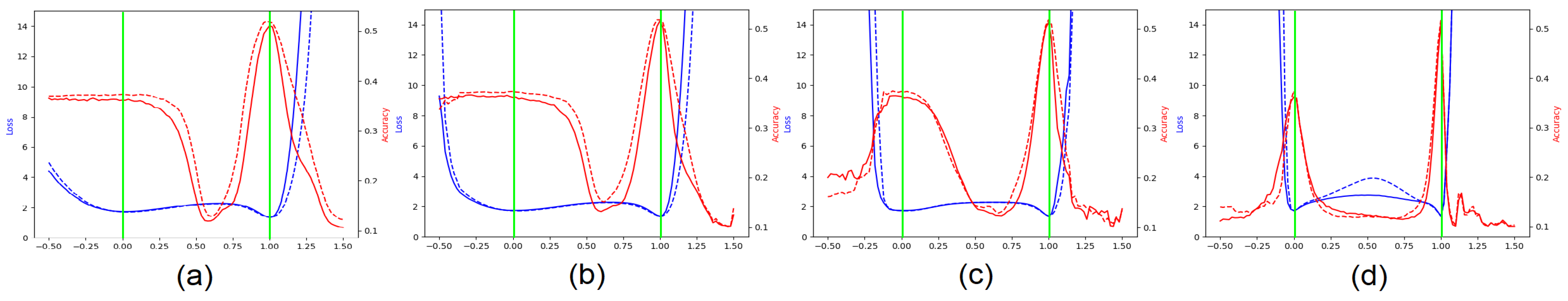
A commonly used method to compare the flatness of two trained networks is to plot the 1D loss/accuracy curves on the interpolation between the two sets of weights. It is also well known that small batch sizes produce flatter minima than bigger batch sizes. We trained on CIFAR-10 a 5 hidden-layer MLP two times, first with a batch size of 8 (network
A) than with a batch size of 1024 (network
B). Then, as performed by [
16], we plotted the 1D loss/accuracy curves on the interpolation between the two weight vectors of the networks (c.f.
Figure 4a). We then performed the same interpolation but between the teleportation of A and B with CoB-ranges
of
,
, and
. As can be seen from
Figure 4, the landscape becomes sharper as the CoB-range increases. Said otherwise, a larger teleportation leads to a locally-sharper landscape. More experiments with other models can be found in
Appendix A.
5. Optimization
In the previous section, we showed that teleportation moves a network along a loss level curve and sharpens the local loss landscape. In this section, we show that teleportation increases the magnitude of the local normalized gradient and accelerates the convergence rate when used during training, even only once. Moreover, we empirically show that this impact is controlled by the CoB-range factor .
We remark that once a neural network is initialized, it is assigned a specific network function and, in principle, a teleported network of this initialized network (which will have the same network function) does not have to train better than the original network and, nevertheless, the teleported network trains better.
In all of our experiments we used L2 regularization and learning rate decay at epoch 80.
5.1. Back-Propagated Gradients of a Teleportation
It has already been noticed by [
2,
5], that under positive scaling of ReLU networks, the gradient scales inversely than the weights with respect to the CoB. Here, we show that the back-propagated gradient of a teleported network has the same property, regardless of the architecture of the network, the data, the loss function and the activation functions.
Let
be a neural network with a set of weights
W and activation functions
f. We denote
the weight tensor of the
ℓ-th layer of the network, and analogously for the teleportation
. The CoB
at layer
ℓ is denoted
, which is a column vector of non-zero real numbers. Let us also consider a data sample
with
the input data and
t the target value and
the gradient of the networks
and
with respect to
the gradient of the loss with respect to W and V at (x,t). Following Equation (
1), we have that
where the operation
multiplies the columns of the matrix
by the coordinate values of vector
, while the operation
multiplies the rows of matrix
by the coordinate values of the vector
.
Theorem 2. Let be a teleportation of the neural network with respect to the CoB τ. Thenfor every layer ℓ of the network (proof in the Appendix A).
If we look at the magnitude of the teleported gradient, we have that
We can see that the ratio
appears multiplying the squared non-teleported gradient
. For an
intra-landscape teleportation,
is randomly sampled from a uniform distribution
for
. Since
are independent random variables, the mathematical expectation of this squared ratio is:
Thus, when
(i.e., no teleportation as described in
Section 4.1), then
, which means that on average the gradients are multiplied by 1 and thus remain unchanged. However, when
, then
, which means that the gradients magnitude is multiplied by an increasingly large factor.
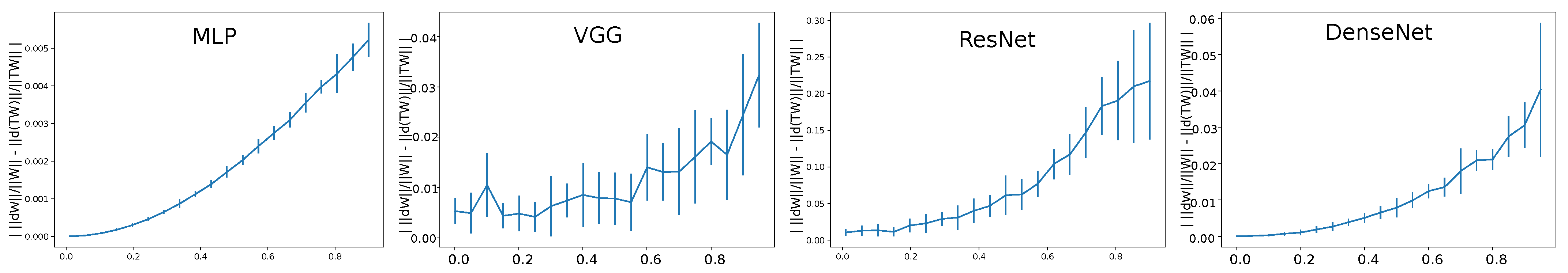
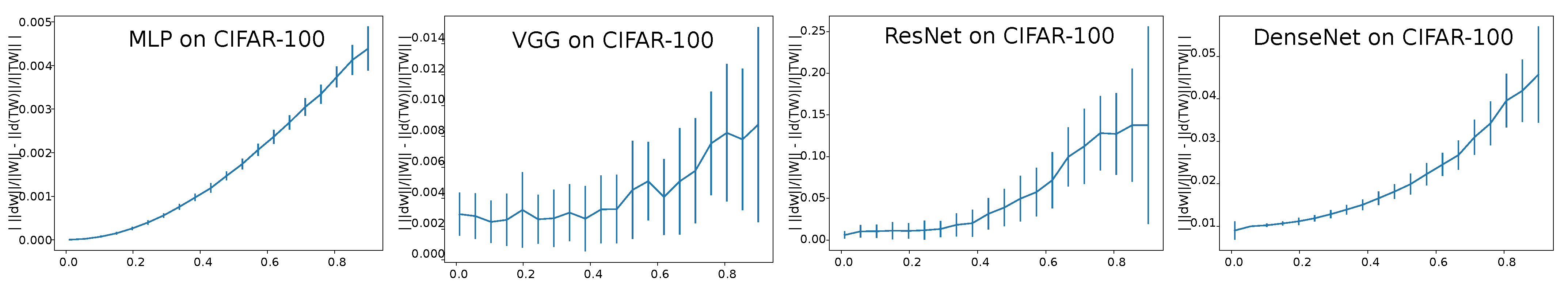
We empirically validate this proposition with four different networks in
Figure 5 (plots for the other models and datasets can be found in the
Appendix A). There we put the CoB-range
on the x-axis versus 20 different teleportations for which we computed the absolute difference of normalized gradient magnitude:
. We can see that a larger CoB-range leads to a larger difference between the normalized gradient magnitudes.
This shows that randomly teleporting a neural network increases the sharpness of the surrounding landscape and, thus, the magnitude of the local gradient. This holds true for any network architecture and any dataset. This analysis also holds true for inter-landscape CoB sampling since the CoB-range appears squared always.
5.2. Gradient Descent and Teleportation
From the previous subsection we obtain that the CoB-range controls the difference on the normalized gradients. Here we empirically show that the CoB-range also has an influence on the training when teleportation is applied once during training.
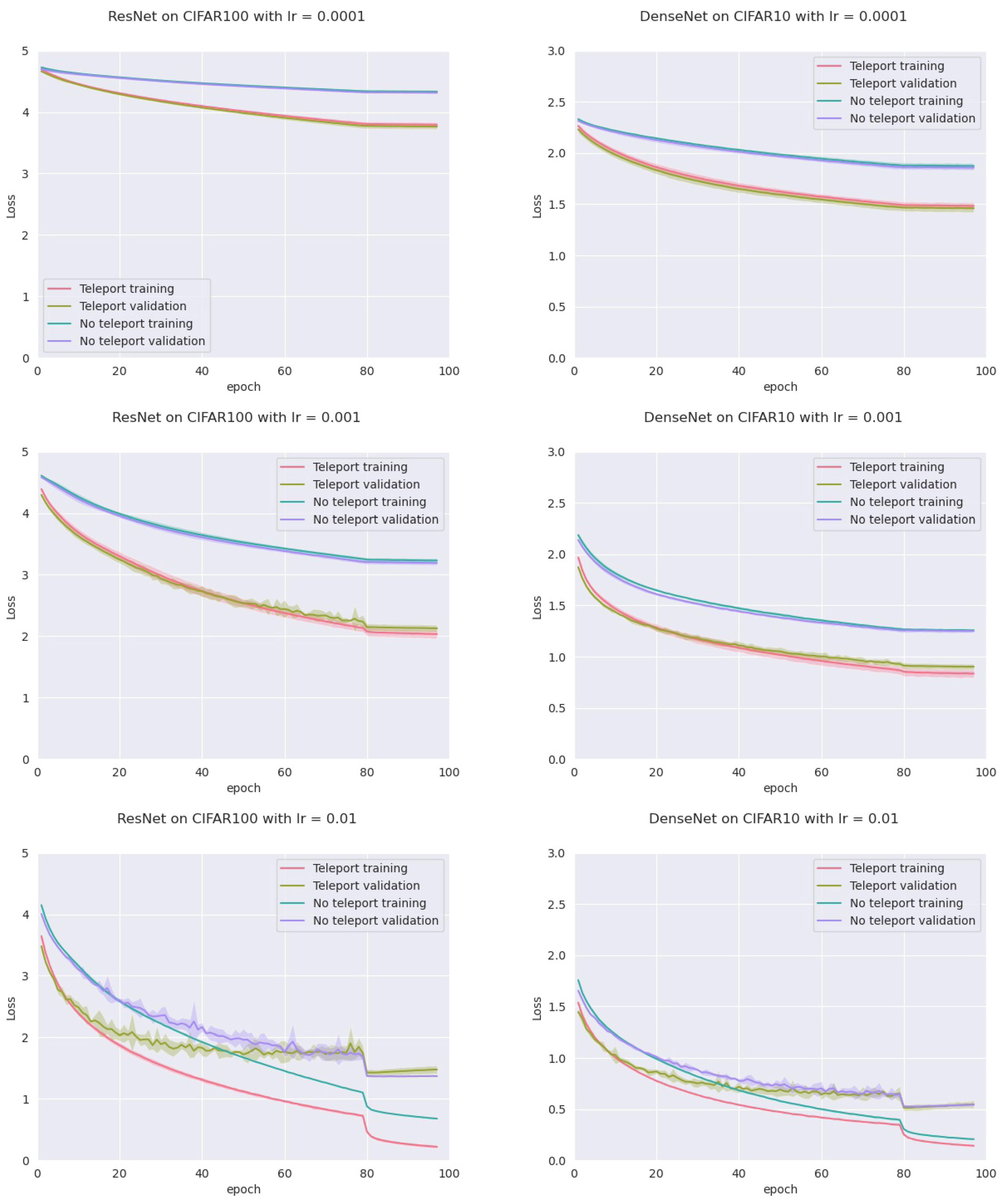
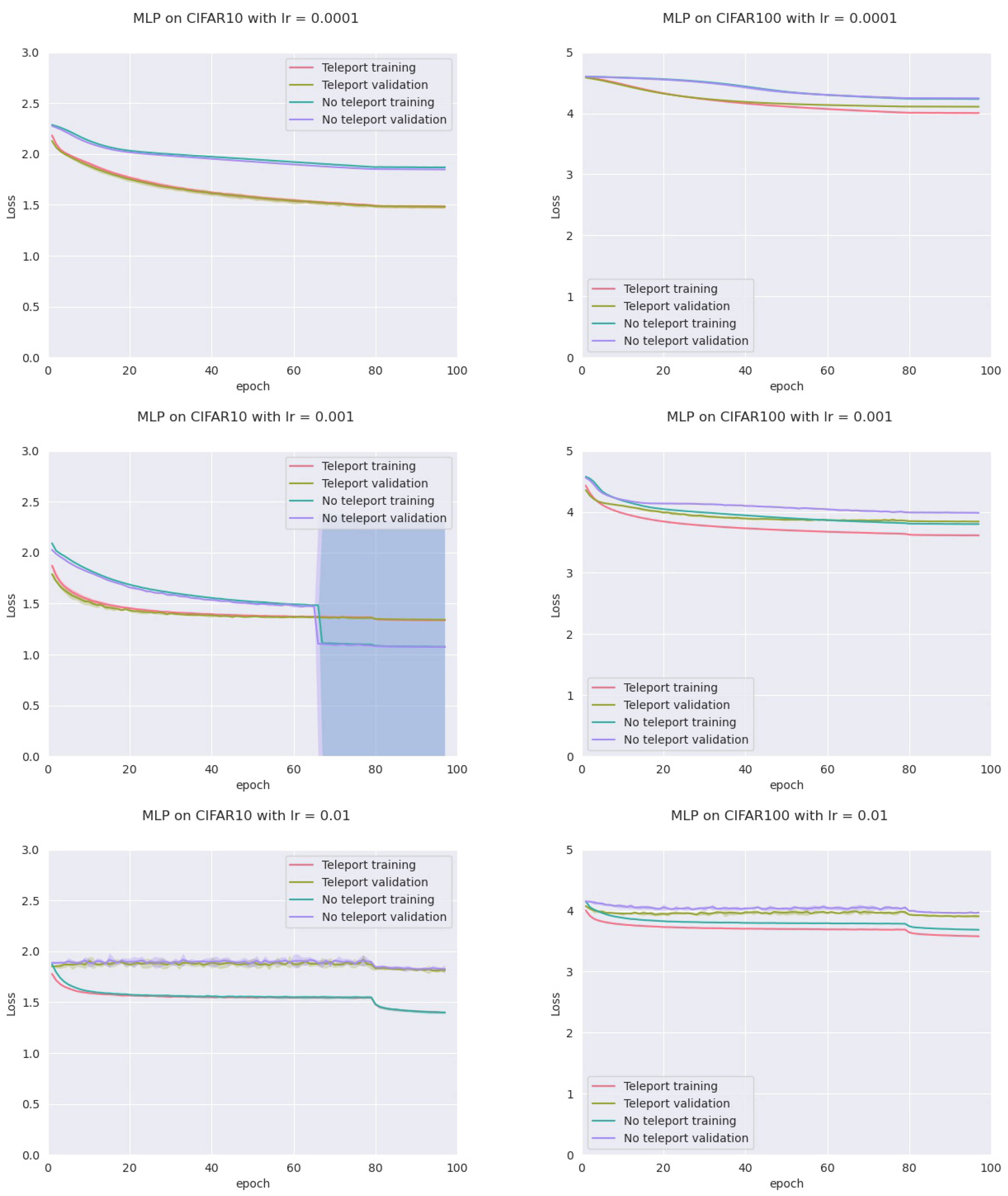
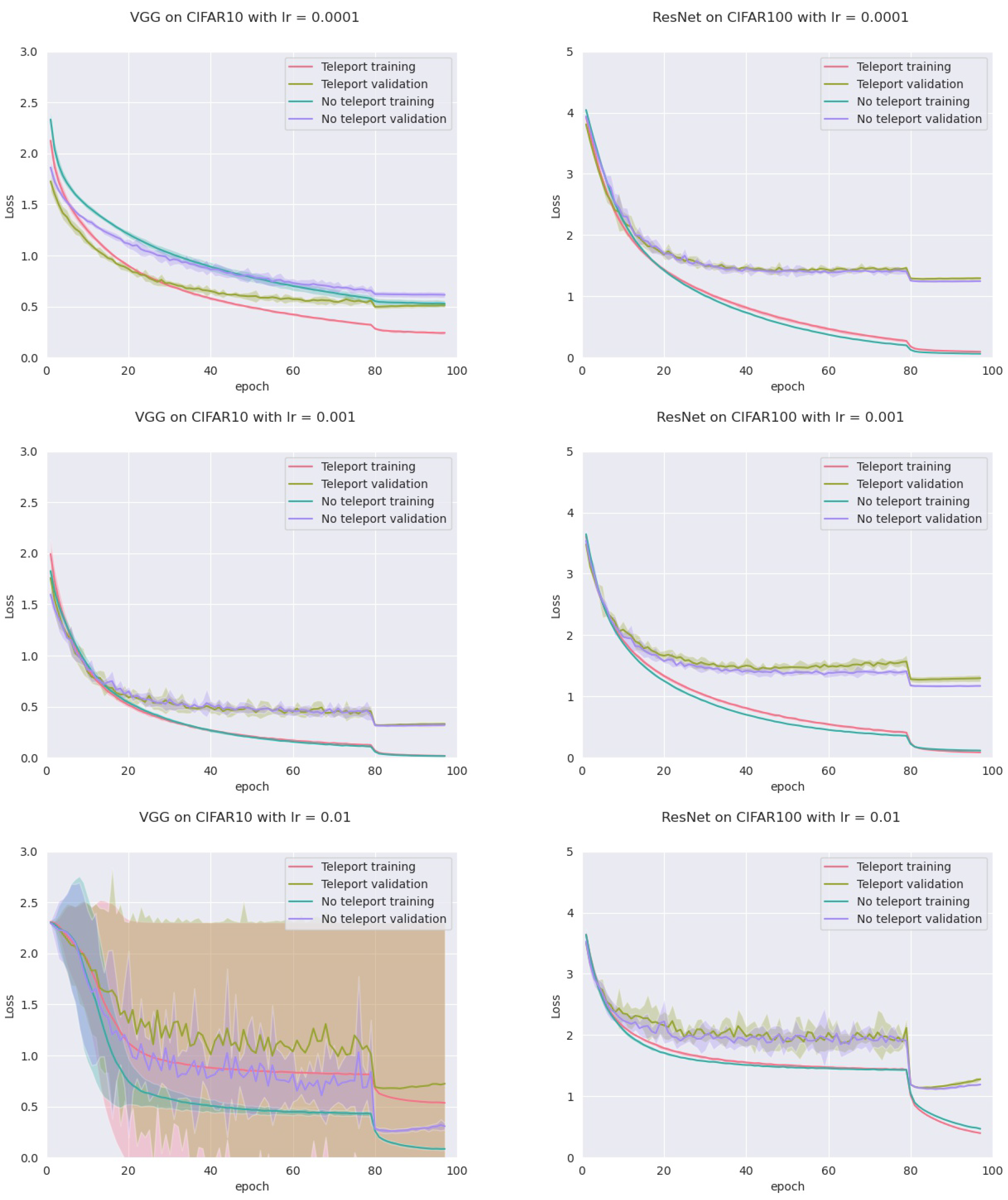
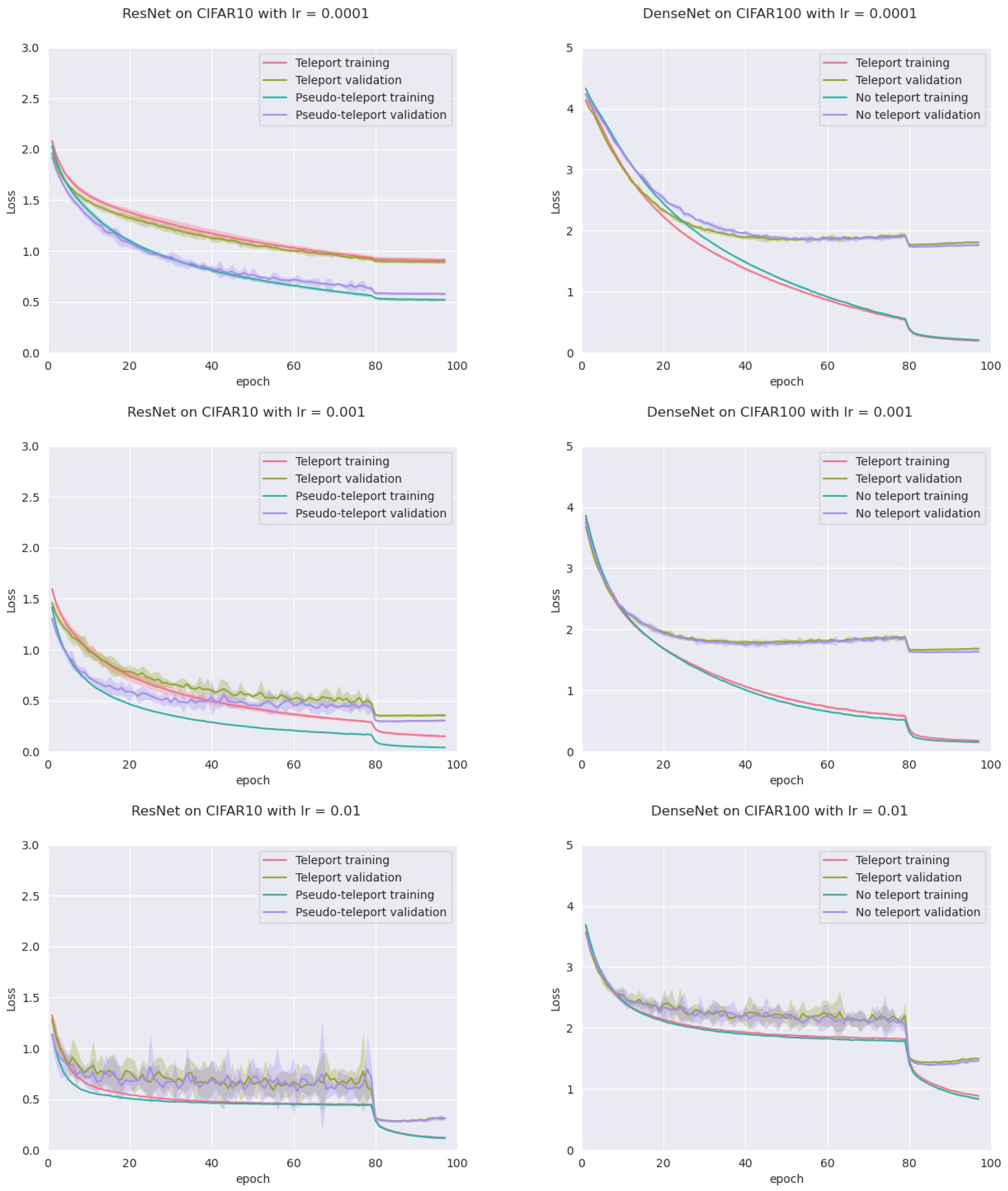
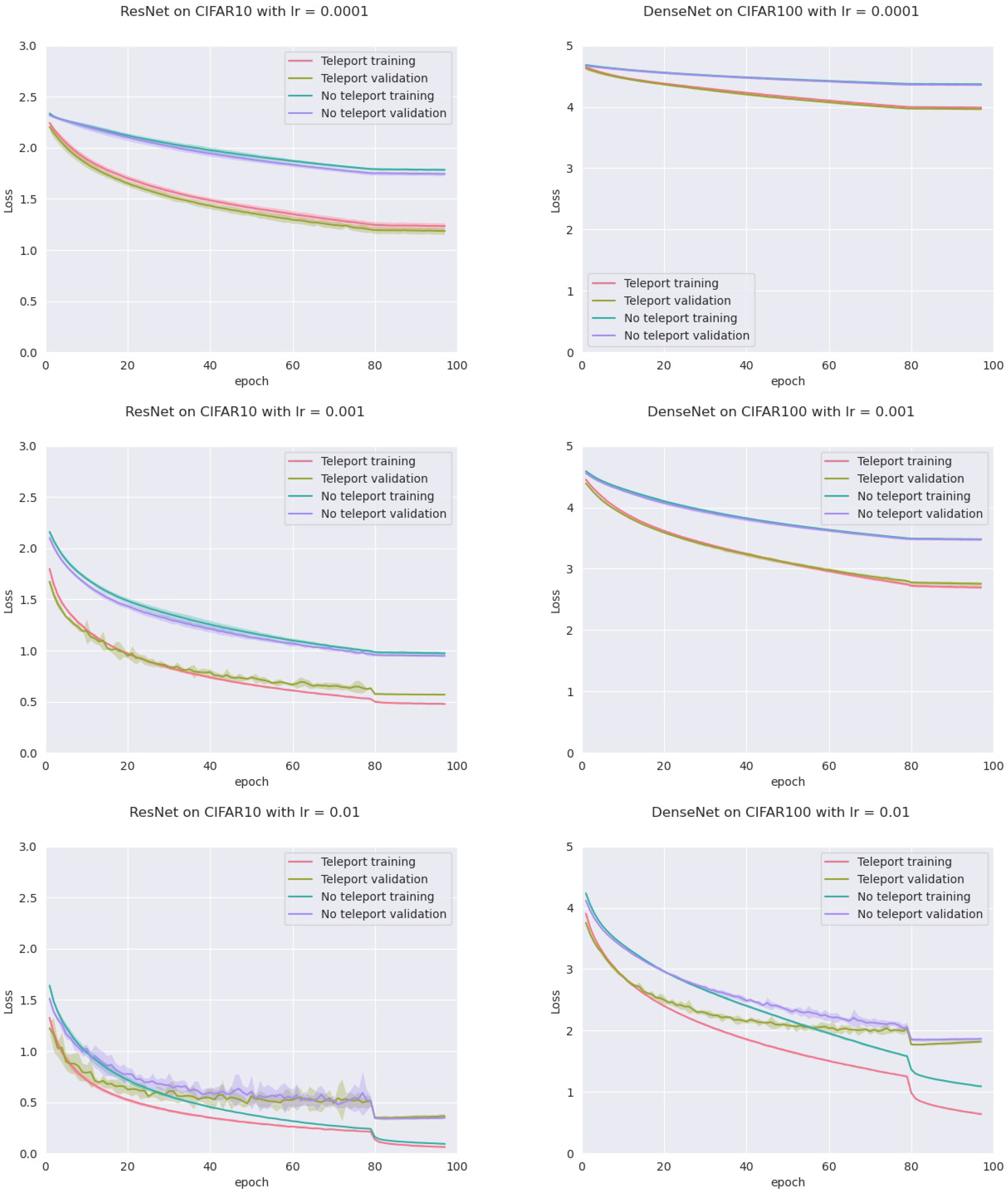
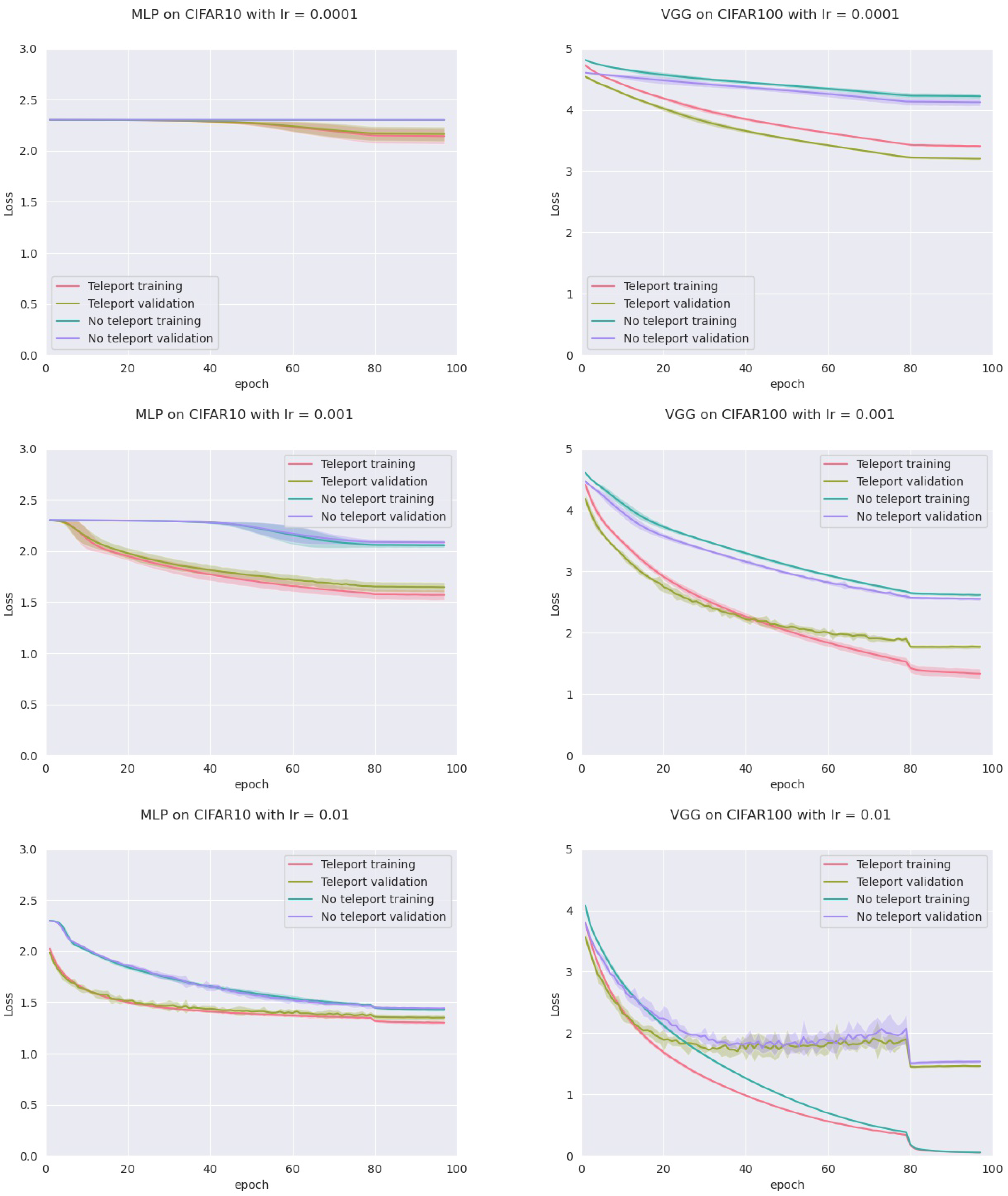
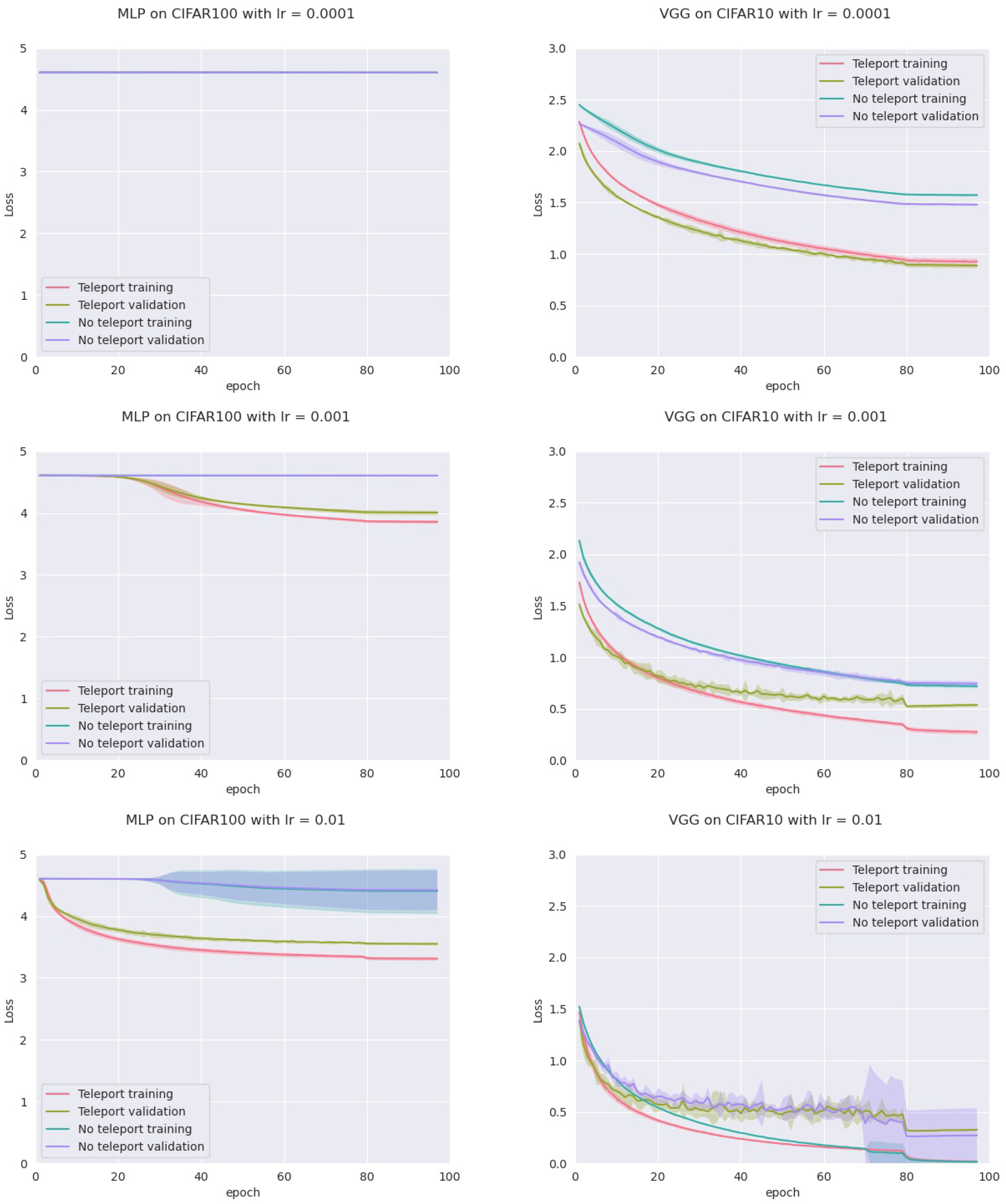
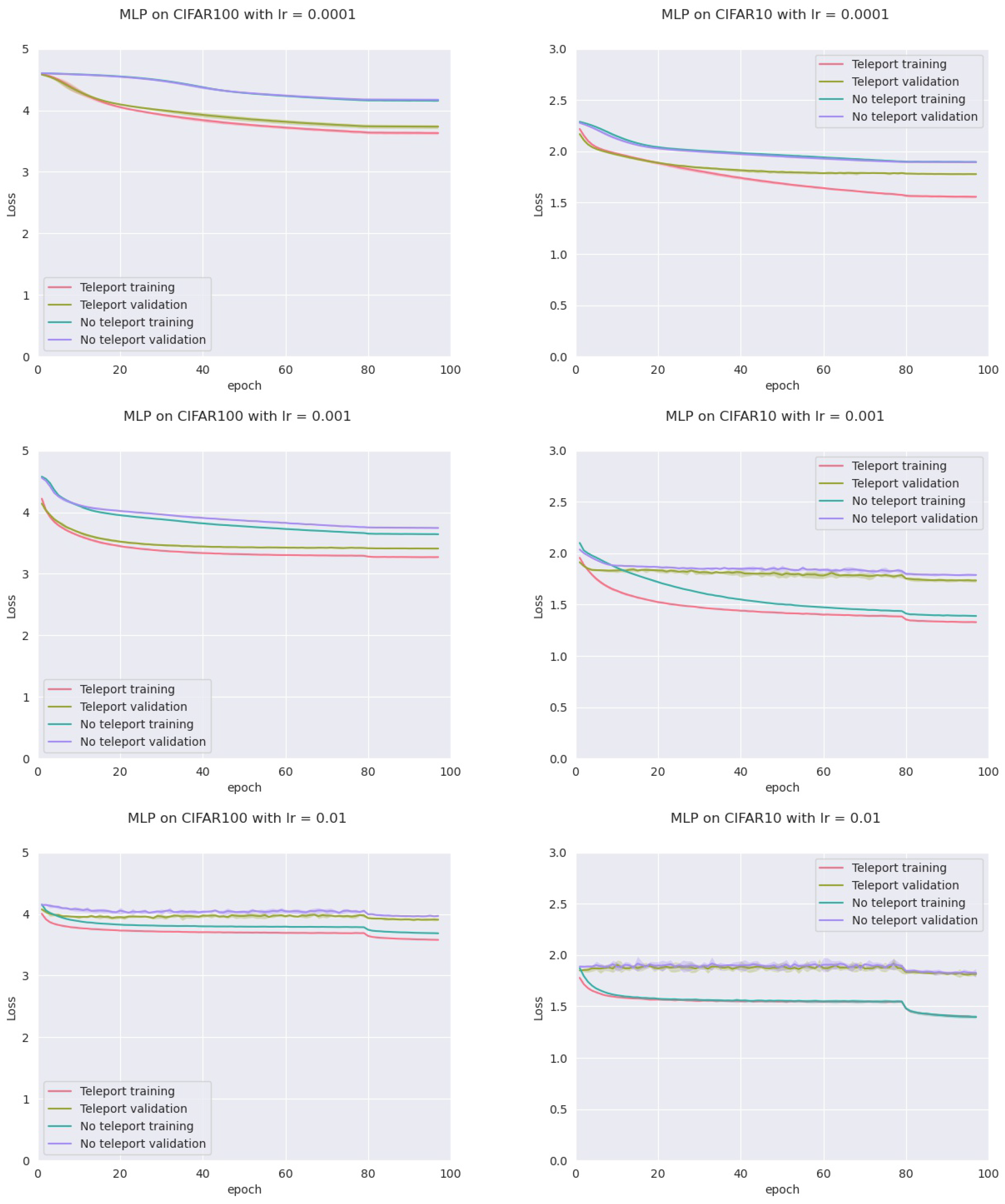
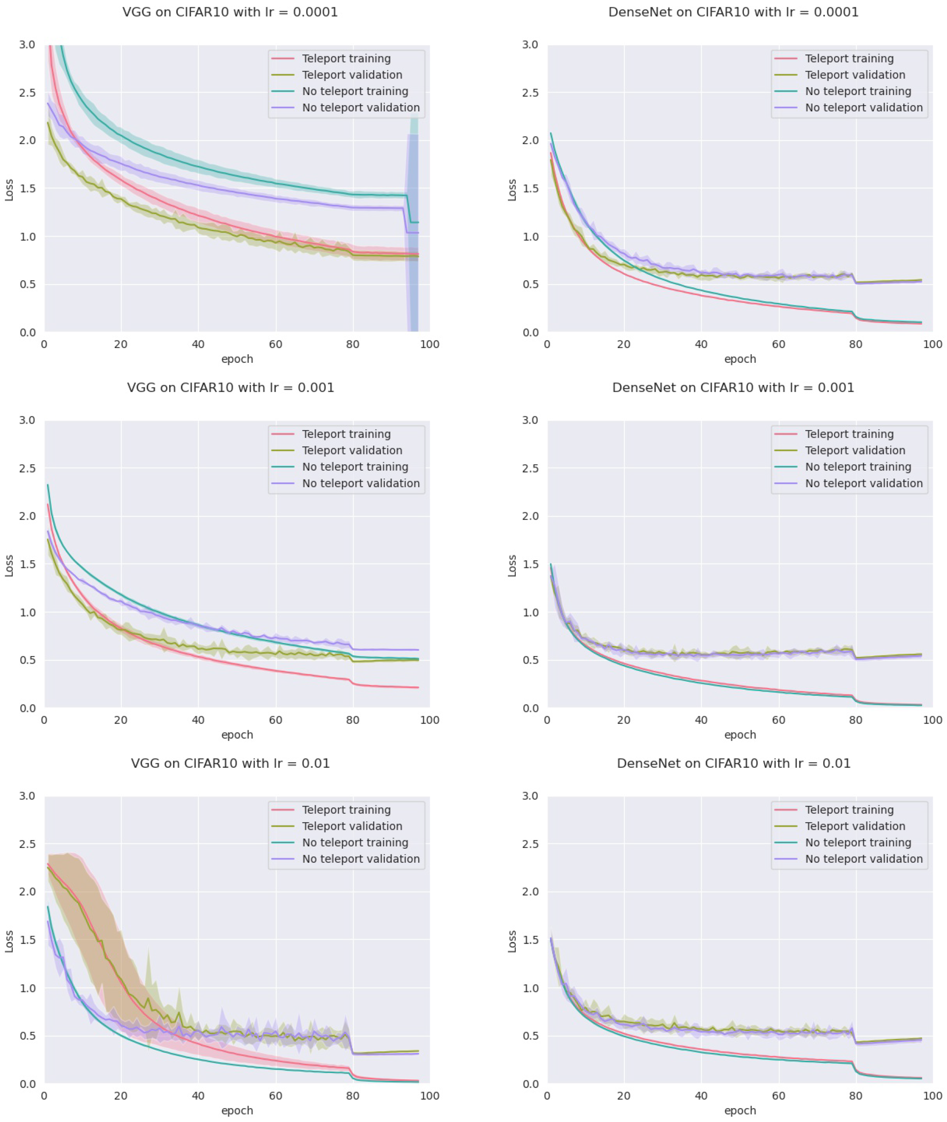
In order to assess this, we trained four models: an MLP with five hidden layers with 500 neurons each, a VGGnet, a ResNet18, and a DenseNet, all with ReLU activation. Training was conducted on two datasets (CIFAR-10 and CIFAR-100) with two optimizers (vanilla SGD and SGD with momentum), and three different learning rates (0.01, 0.001 and 0.0001) for a total of 72 configurations. For each configuration, we trained the network with and without neural teleportation right after initialization. Training was performed five times for 100 epochs. The chosen CoB range is with an inter-landscape sampling for all these experiments. The teleported and non-teleported networks were initialized with the same randomized operator following the “Kaiming” method.
This resulted into a total of 720 training curves that we averaged across the learning rates (±std-dev shades), see
Figure 6 (plots for the other models and datasets can be found in
Appendix A). As can be seen, neural teleportation accelerates gradient descent (with and without momentum) for every model on every dataset.
To make sure that these results are not unique to ReLU networks, we trained the MLP on CIFAR-10 and CIFAR-100 with three different activation functions: LeakyReLU, Tanh and ELU, again with and without neural teleportation after the uniform initialization, which is the default PyTorch init mode for fully connected layers. As can be seen from
Figure 7 (plots for the other models and datasets can be found in
Appendix A), here again,
one teleportation accelerates gradient descent (with and without momentum) across datasets and models.
In order to measure the impact of the initialization procedure, we ran a similar experiment with a basic Gaussian initialization as well as an Xavier initialization. We obtained the same pattern for the Gaussian case; for the Xavier initialization, teleportation helps the training of the VGG net, while for the others the difference is less prominent, see
Figure 8 (plots for the other models and datasets can be found in
Appendix A).
Given a neural network
W, we produced another one,
V, by first teleporting
W to
and then sampling
V from the sphere with center
W and radius vector
. We called this a
pseudo-teleportation. We then trained the four models with the same regime, comparing pseudo-teleportation to no teleportation. Results in
Figure 9 reveal that pseudo-teleportation does not improve gradient descent training (plots for the other models and datasets can be found in
Appendix A).
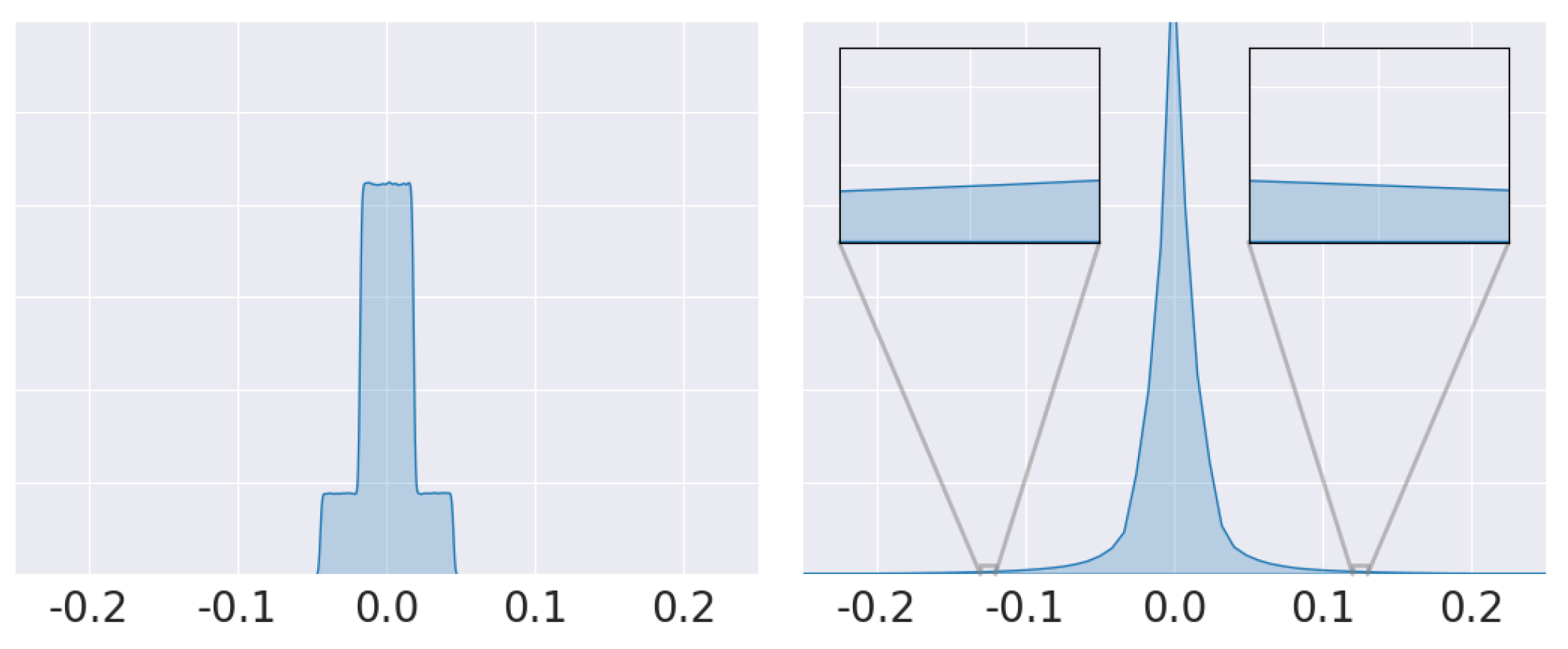
We show in
Figure 10 the weight histograms of an MLP network initialized with a uniform distribution (PyTorch’s default) before (left) and after (right) teleportation.
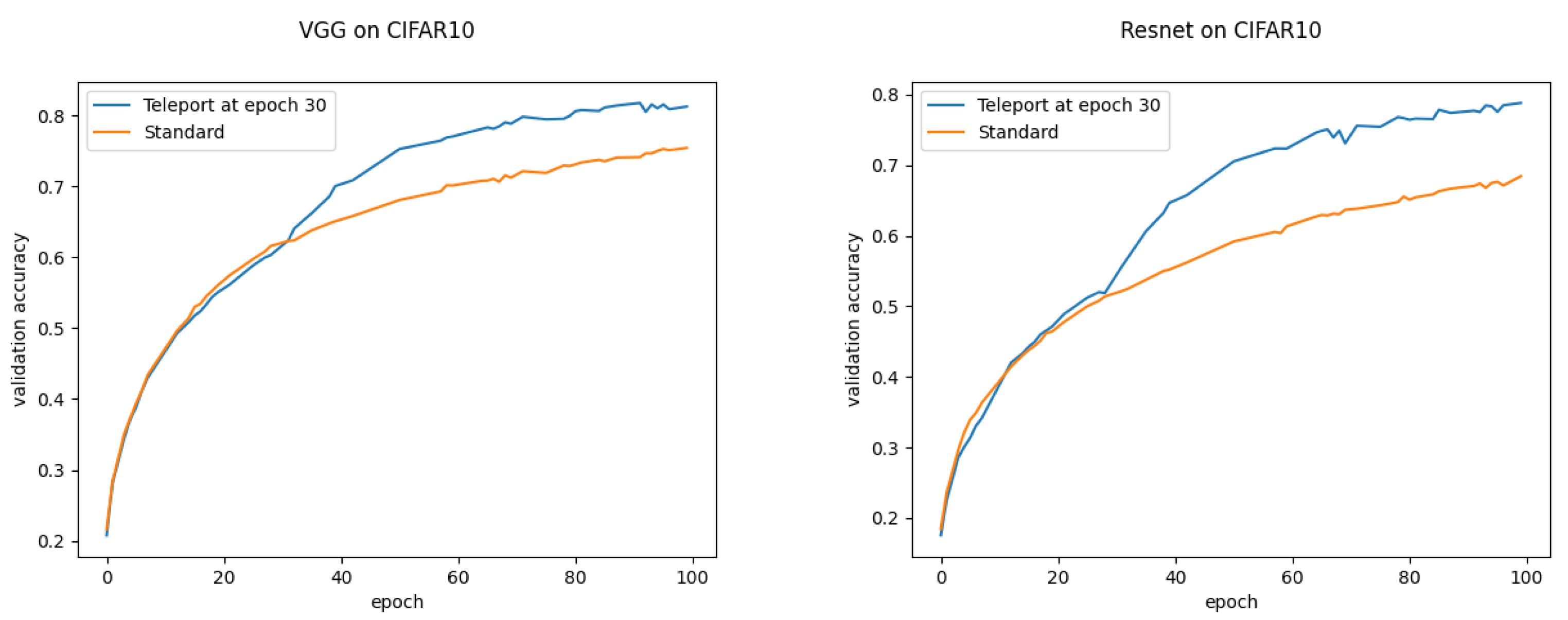
For all the previous experiments, we teleported the neural networks at the beginning of the training. Finally, we performed another set of experiments by teleporting the neural network once at epoch 30. We can clearly see the jump in accuracy right after the teleportation in
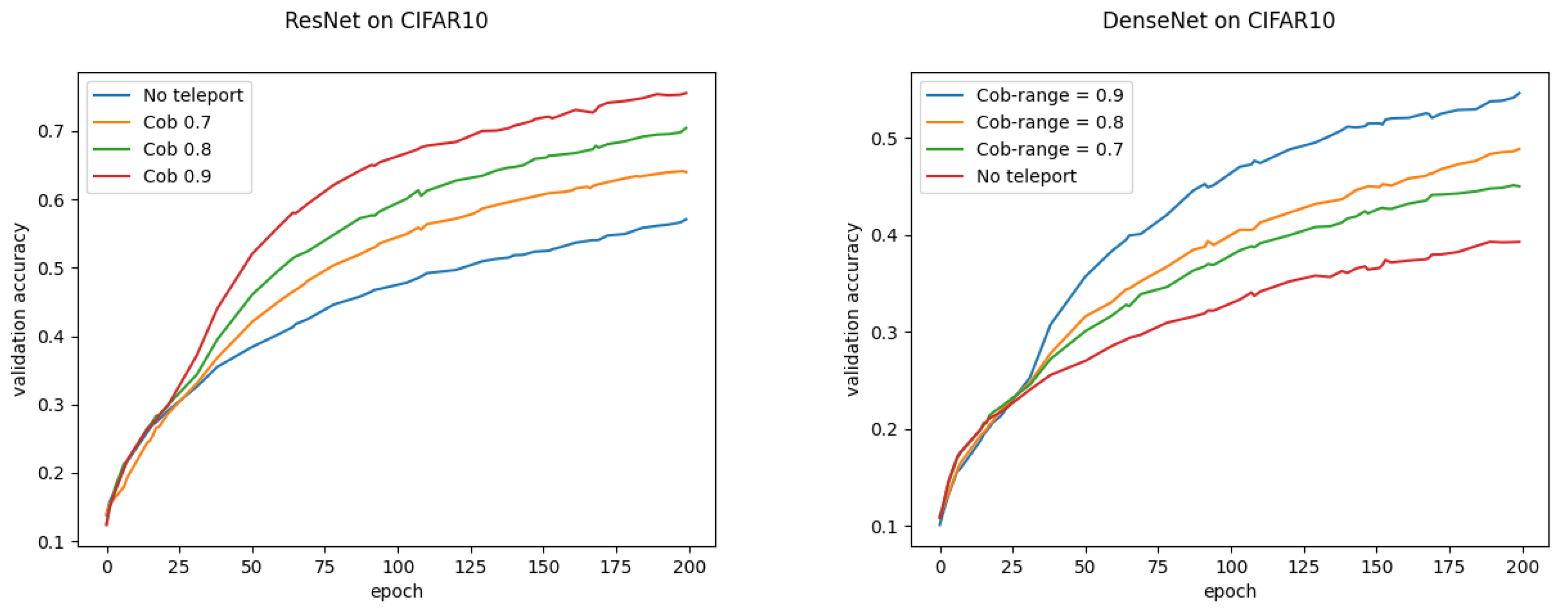
Figure 11. In
Figure 12, we compare the training curve of a model with a training where we teleport once at epoch 30 with different CoB-ranges of
,
and
. We can see how the bigger the Cob-range, the higher the impact on validation accuracy. Experiments shown in
Figure 11 and
Figure 12 were run with a learning rate of
on CIFAR-10.
6. Conclusions
In this paper, we provided empirical evidence that neural teleportation can project the weights (and the activation functions) of a network to an infinite amount of places in the weight space while always preserving the network function. We show that: (1) It can be used to explore loss level curves; (2) Micro-teleportation vectors are always perpendicular to back-propagated gradients (
Figure 3); (3) teleportation reduces the landscape flatness (
Figure 2) and increases the magnitude of the normalized local gradient (
Figure 5 and
Figure 12) proportionally to the CoB range
used, and (4) applying
one teleportation during training accelerates the convergence of gradient descent with and without momentum (
Figure 6,
Figure 7,
Figure 8 and
Figure 11).
Although teleportation looks only like a trick to preserve the network function by just rescaling the weights and the activation functions, it is more than a trick as (i) it comes from the foundational definitions and constructions of representation theory, which neural networks exactly satisfy, and (ii) it has unexpected properties on neural network training when applied once. The latter underlines the fact that we really do not know the landscape of neural networks and that more tools (or new mathematics) are needed for further understanding. Moreover, in principle, a neural network and its teleportation should train very similarly, since they both have the same network function, and we have demonstrated that this is not the case.
We conclude that neural teleportation, which is a very simple operation, has remarkable and unexpected properties. We expect these phenomena to motivate the study of the link between neural networks and quiver representations.
Finally, we acknowledge that several different types of change of basis sampling can be performed instead of the uniform distribution around 1 and that we have chosen. In any case, if there are other types of change of basis sampling for which the properties of interest do not hold, then we ask: what makes uniform sampling different?


 ,
, 


