1. Introduction
Neural network quantization is a field of study that focuses on improving the speed of neural network inference by using integer weights and/or activations. This field encompasses algorithms for training and running quantized neural networks (QNNs). Recent research has proven that the gap in quality between QNNs and full precision models is negligible in many tasks [
1,
2,
3]. In addition to achieving high quality, practical applications also demand the computationally efficient inference of QNNs in various environments. Data-processing centers tend to rely on tensor processors and specialized accelerators [
4,
5,
6], which greatly benefit from QNNs. However, edge devices such as mobile phones and smart gadgets often perform computations on central processing units (CPUs) [
7,
8,
9,
10], which have limited computational resources and sometimes are not able to provide high processing speed.
The most computationally challenging operation in neural networks is matrix multiplication. Both convolutional and fully connected layer computations usually rely on matrix multiplication. Thus, the implementation of QNNs is primarily focused on developing specialized algorithms for quantized matrix multiplication. CPUs have a predefined general-purpose architecture, which imposes significant constraints on the algorithm design.
In this work, we propose a novel parametric quantization scheme called 4.6-bit quantization aimed to provide fast inference on CPUs. This scheme is designed to be a faster alternative to eight-bit QNNs on low-power (e.g., mobile and embedded) devices, and outperform four-bit models in terms of recognition quality. To achieve it, we restrict signed products of weights and activations by the eight-bit register capacity and obtain corresponding ranges for weights and activation values. With such an approach, these ranges are not limited to the powers of two and provide more quantization bins than ranges of four-bit quantization. Because the 16-bit accumulators of 8-bit products restrict the multiplication depth, we perform a two-stage summation with 16- and 32-bit accumulators. All the operations are vectorized via SIMD (Single Instruction Multiple Data) CPU extension. We develop a high-performance implementation for ARM (the processors of choice for mobile and embedded devices) and x86 CPUs (the most popular processor architecture used in modern desktop computers). We also perform an experimental evaluation of the efficiency of the proposed quantization method.
We demonstrate the recognition quality achieved by 4.6-bit QNNs on CIFAR-10 and ImageNet datasets and the semantic segmentation quality on the TCIA dataset. The proposed scheme is parametric, with a parameter that governs the balance between the number of quantization bins for weights and activations. We observe this trade-off and identify the best balance of quantization bins for QNNs.
Thus, our contribution is as follows:
We propose a new quantization scheme called 4.6-bit quantization. This scheme offers higher accuracy than 4-bit quantization while preserving the same computational efficiency on CPUs.
We present an algorithm for computationally efficient 4.6-bit quantized matrix multiplication specialized for ARM and x86 CPUs.
We demonstrate a way to build neural networks based on the proposed quantization scheme and matrix multiplication algorithms.
We experimentally evaluate the computational efficiency of the proposed matrix multiplication and prove that it is 1.9–2 times faster than floating-point matrix multiplication on ARM and x86 CPUs. It is also 1.7 and 1.3 times faster than ten eight-bit matrix multiplication ARM and x86 CPUs, respectively. The proposed quantization is especially interesting for fast and accurate QNN inference on mobile devices.
We conduct experiments on 4.6-bit QNN prediction accuracy and compare it to eight-bit and four-bit QNNs. These experiments prove that 4.6-bit quantization is noticeably more accurate than the four-bit one, while their computational demands are comparable. They can also serve as an illustration of how to train arbitrary 4.6-bit networks.
The rest of this paper is organized as follows.
Section 2 provides a brief overview of related works. In
Section 3, we describe neural network quantization from the computational point of view.
Section 4 presents our quantization method, and
Section 5 demonstrates its experimental evaluation. In
Section 6, we discuss the limitations and impact of our work. Finally,
Section 7 concludes our work.
2. Related Works
QNNs are widely used on CPUs. For instance, an efficient implementation of 8-bit networks with 8-bit weights and 32-bit accumulators accelerated using Single Instruction Multiple Data (SIMD) instructions was introduced in [
11].
Nowadays, there are even more efficient implementations for eight-bit quantized networks, such as Google’s gemmlowp [
12], ruy [
13], Tensorflow [
14] and Facebook’s qnnpack [
15] libraries. There are modern ARM CPUs that have instructions specifically designed for machine learning purposes. These instructions can noticeably speed up eight-bit QNN inference [
16]. Fast implementations are also available for ternary [
17,
18,
19] and binary networks [
18,
20]. However, binary and ternary networks still suffer from accuracy loss compared to full-precision or eight-bit quantized networks with a similar number of parameters and architecture, which limits their suitability for certain tasks.
Furthermore, training methods for low-precision QNNs are being actively developed. One promising approach is post-training quantization (PTQ), which involves quantizing an already trained floating-point neural network [
21,
22]. Notably, recent research [
22] has demonstrated the ability to train four-bit networks for some tasks with minimal accuracy loss. Additionally, there is an ongoing development of quantization-aware training (QAT) techniques for scenarios where training data are available [
23,
24]. These approaches show significant potential for advancing the field of computationally efficient recognition and facilitating the implementation of QNNs in practical applications.
Fast implementations of low-precision QNNs have also successfully been developed. For instance, in our previous work [
25] we introduced an algorithm for four-bit quantized multiplication on ARM CPUs that works faster than the eight-bit algorithm. However, it has limitations in handling large neural networks due to constraints on multiplication depth. Won et al. [
26] proposed a packing method that allows for placing several inputs or weights into one register and processing them in multiplication together, increasing its efficiency. Cowan et al. [
27] perform a search for an efficient instruction sequence to implement low-precision matrix multiplication. However, these approaches require additional steps for both packing and unpacking, and only consider integer values for bits per weight.
3. Quantization Background
3.1. General Quantization Scheme
During the quantization process, floating-point values are approximated by integer ones. That is performed to reduce memory footprint and simplify computations. The quantization scheme presented in [
28] is based on the affine mapping between integer value
q and real
r:
where the real-valued scale factor (
S) and the integer-valued zero-point (
Z) are parameters of quantization. Google’s gemmlowp [
12] and Facebook’s qnnpack [
15] libraries use this scheme to map the real values of matrices to eight-bit unsigned integers as follows:
where
stands for rounding to the nearest integer,
,
(for eight-bit quantization). In [
25,
29,
30], the authors use the same scheme for four-bit quantization (
,
).
3.2. Quantized Matrix Multiplication
Let us consider matrix multiplication of two real-valued matrices:
in which matrices
A and
B are approximated with integer matrices
and
using (
2) with parameters
,
and
,
, respectively. In this case
C can be approximated by
with scale
and zero-point
:
We can see that
can be computed with integer-only arithmetic. Some algorithms for quantized multiplication directly apply Equation (
4), while others use the following approach:
where the first term is the matrix multiplication of quantized matrices, the second and the third are easy to compute (as they require a single matrix each), and the fourth is constant.
So, to compute a network efficiently, we need to define a fast algorithm for the multiplication of quantized matrices and quantization parameters (
S and
Z) for the inputs and weights of each neural network’s layer. There exist several strategies for choosing quantization parameters. They can be set to match the whole range of possible values [
28], set to quantize weights and inputs with minimum error [
29,
30], or directly learned during network training process [
1].
3.3. High-Performance Matrix Multiplication
The major part of QNN inference on CPUs is matrix multiplication. It is required for implementations of fully connected and convolutional layers, as a convolution in neural networks is usually transformed into the matrix multiplication using im2col or similar algorithms [
31,
32,
33].
In order to achieve optimal matrix multiplication performance, it is crucial to consider data locality and make efficient use of cache memory. The sizes of the caches are limited, so matrix multiplication algorithms usually load small blocks of
m rows from a left matrix and
n cols from a right matrix, store values in a specific order, and provide a highly optimized function (which is called microkernel), that computes the matrix product of them with a size
. The result is accumulated directly in CPU registers, as blocks should be small enough to fit into caches [
34].
SIMD extensions are often used in the microkernel to provide maximum performance. ARMv8 processors have 32 128-bit registers. Each of them can hold 4 32-bit integers or floating-point values each, 8 16-bit values, or 16 8-bit values.
For example, for 4-bit efficient matrix multiplication, 16 4-bit values can be stored as 16 8-bit values in the SIMD register, then UMLAL and UMLAL2 instructions are applied to multiply and accumulate them into a 16-bit register [
25]. However, 16-bit accumulators pose restrictions on the depth of matrix multiplication, so the algorithm could only be applied to small QNNs.
4. 4.6-Bit QNN
4.1. 4.6-Bit Quantization
The key feature that allowed for the acceleration of the 4-bit multiplication algorithm [
25] in comparison to the 8-bit algorithm [
12] is that it multiplied 8-bit values (16 per 128-bit SIMD register) instead of 16-bit values (8 per SIMD register) and accumulated results in 16-bit accumulators instead of 32-bit accumulators. That is possible because the product of four-bit values (i.e., quantized value
q from Equation (
2) satisfies inequality
) fits into the eight-bit register.
Let us consider the signed multiplication of two quantized values
x and
w that fit into a signed eight-bit integer product:
This scheme allows for
quantization bins for
x and
quantization bins for
w, where
There are 21 pairs
which satisfy (
6): (255, 3), (127, 5), (85, 7), (63, 9), (51, 11), (43, 13), (37, 15), (31, 17), (29, 19), (25, 21), (23, 23) and symmetrical ones. If we compute the average bitwidth required to store
x and
w as
, we obtain values in the range 4.51–4.79. So, we name this scheme 4.6-bit quantization.
In
Figure 1, we demonstrate how the three considered quantization schemes use CPU registers. Note, that both four- and 4.6-bit schemes do not use the full capacity (256 possible values) of the eight-bit register. However, this overhead only occurs during the inference of the network, i.e., in random access memory (RAM) and CPU registers, and is required for the sake of performance. When we store the network in secondary memory (e.g., hard drive), we can use compression algorithms to ensure that the network size is small.
We can see that that the proposed scheme allows for more quantization bins than four-bit quantization, for which . It results in a higher accuracy approximation of floating-point multiplication with the quantized one, while preserving the same computational efficiency (the only difference is that unsigned operations are replaced by signed).
It should be emphasized that despite the fact that the quantized values in our case are zero-symmetric (
), it does not limit the applicability of the proposed scheme to zero-symmetric distributions. For example, let us assume that the input is uniformly distributed in the range
(
). For quantization with
bins, the following parameters are applied:
,
,
, and
according to Equation (
1). The quantized values
, 0, and 11 represent the real values 0,
, and 1, respectively.
Our proposed 4.6-bit is a special case of the uniform quantization schemes (presented in
Section 3.1). Thus, it has a higher approximation error than nonuniform ones (e.g., quantization of LQ-Nets [
35]). However, that is the price for the performance provided by the ability to directly multiply the quantized values in order to compute matrix multiplications (
3) and (
4).
4.2. Memory Footprint
The memory footprint of QNNs is a crucial aspect of their practical applications. In the context of our proposed 4.6-bit quantization and the four-bit quantization in [
25], quantized values are stored in eight-bit registers. It implies that weights and activations occupy the same amount of memory in RAM for a fixed network architecture for four-bit, 4.6-bit, and eight-bit QNNs.
The output values of a layer in our 4.6-bit QNNs are represented as 32-bit integers, consistent with 8-bit QNNs. However, in the case of the 4-bit quantized layer in [
25], the outputs are 16-bit integers. This introduces a limitation on the multiplication depth that we will explore further in the subsequent section.
Note that linear operations in a layer can be fused with activation for computational and memory efficiency, resulting in an 8-bit output as suggested in [
28]. Therefore, all the considered QNNs exhibit nearly identical memory footprints in RAM, and this footprint is four times smaller than that of 32-bit floating-point networks.
However, if we consider the storage of the network in the secondary memory (e.g., hard drive), the network weights can be stored using data compression techniques (e.g., Huffman coding [
36]). Thus, we can achieve significant compression. Even under the assumption of uniform weight distribution, the memory footprint approaches
, where
is the number of quantization bins of the weights. Therefore,
allows us to control secondary memory consumption, which is essential for mobile applications.
Furthermore, the actual distribution of weights in the network is not uniform. Let us consider 4.6-bit quantized U-Net from our experiments in
Section 5.5.
Figure 2 illustrates the weight distribution in this model, revealing a significantly higher frequency of values close to zero compared to those near
(
, and thus quantized weights values belong to
). Therefore, Huffman coding results in an even more substantial compression rate (e.g., 3.02 bits per element in that particular case).
4.3. Matrix Multiplication
Let us consider quantized matrix multiplication (
5). In our particular case, the right matrix is the matrix of neural network weights. Weight distribution in the trained neural network is usually zero-symmetrical [
37], as is the range of possible values in our quantization scheme. That is why we set the zero-point or the right matrix
to constant zero. Thus, Equation (
5) can be significantly simplified:
Then, we can compute the sums over columns of offline (after the network training but before its inference). At the inference time, we only need to multiply them by and subtract them from the bias (which is also added channel-wise in the neural network).
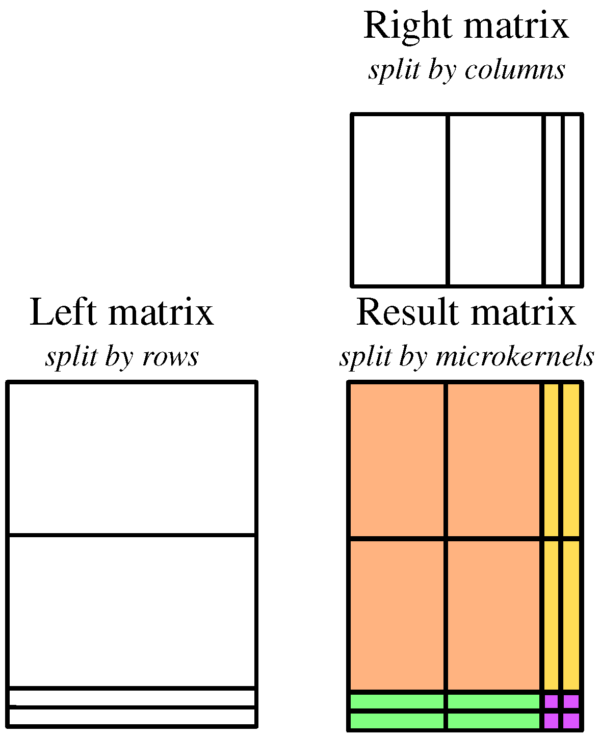
Matrix multiplication is computed by
microkernels—high-performance functions as mentioned in
Section 3.3. For the microkernel to be applied, the left and right matrices should be split: blocks of
m rows are extracted from the left matrix, and blocks of
n columns are extracted from the right matrix. The values in the blocks are reordered so that the loads from those blocks during the
microkernel application are sequential in memory. It decreases the number of cache misses and thus accelerates matrix multiplication on CPUs [
34]. A simplified version of the matrix split is illustrated in
Figure 3. In practice, blocks of the left and right matrices are additionally limited in depth dimension (number of columns in the left block and rows in the right block). This is performed so that blocks fit into the cache memory, and the result is accumulated in CPU registers [
34].
Note that we can perform reordering blocks in the matrix of weights (in our case, the right matrix) required for microkernel offline because the network weights do not change during inference. On the contrary, the network inputs (and thus the left matrix of matrix multiplication) vary. Thus, the left matrix has to be reordered at the inference time. Note that when performing matrix multiplication, there is a need for extra memory to store the rearranged blocks of the left matrix. Fortunately, this amount is small enough (no more than m rows) and can be allocated only once and reused.
Thus, the main component of quantized matrix multiplication is the microkernel, which performs the most computations in the matrix multiplication and, therefore, in the QNN in general. Let us consider the 4-bit quantized matrix multiplication algorithm presented in [
25]. It works as follows:
Loads four-bit values (numbers in the range ) from the left and right blocks, stored in eight-bit registers;
Multiplies them using SIMD vector instructions, which perform the same operation over several values simultaneously (in that particular case, over 16 8-bit values packed into 128-bit registers);
Accumulates the result in unsigned 16-bit values in SIMD registers.
This algorithm has an important limitation regarding the depth of matrix multiplication, which ensures that computations are free of overflow issues. The values of the left and right blocks are in the range ; thus, the element-wise products are in the range . Therefore, the sum of more than such values may overflow the register and lead to incorrect results.
The proposed multiplication algorithm for 4.6-bit QNNs is very similar to the 4-bit one but with the following differences:
Due to additional load/store instructions in the outer loop and a larger memory footprint, the considered algorithm is slightly less computationally efficient than four-bit matrix multiplication [
25] but still significantly faster than eight-bit matrix multiplication. We experimentally show that in
Section 5.
4.3.1. ARM NEON Microkernels
To implement the proposed 4.6-bit microkernel on a specific CPU, we need to consider its instruction set and the number of available SIMD registers. The latter determines the microkernel shape. Let us now consider ARMv8-A CPUs, which have 32 128-bit SIMD registers.
The main microkernel for 4.6-bit matrix multiplication on ARM, which has a size of , is presented in Algorithm 1. This size allows for the usage of 24 128-bit SIMD registers as 192 16-bit accumulators ( in Algorithm 1). Another four registers ( and b) are used to read 4.6-bit quantized inputs, stored in eight-bit values. Finally, four registers () are used in intermediate computations to hold the broadcast values from the weight matrix. That is how we use all the 32 SIMD registers available.
In the Algorithm 1 pseudocode, we use ARM intrinsic functions to simplify the algorithm description. However, in practice, we used assembly code to ensure that all registers were used efficiently. We also implemented , , , and (dot product) microkernels. That allowed us to compute matrix multiplication of matrices with arbitrary sizes.
4.3.2. x86 SSE Microkernels
Modern x86 CPU architecture also supports SIMD extensions, e.g., SSE (Streaming SIMD Extensions), AVX (Advanced Vector Extensions), AVX2, AVX-512, etc. Here, we will consider SSE, which supports 16 128-bit SIMD registers.
| Algorithm 1: 4.6-bit microkernel using ARM intrinsics. |
Input: k—depth of matrix multiplication; A—8-bit integer left matrix block stored in specific order: (1) The first 8 values from the first column; (2) The first 8 values from the second column; (3) The same for the next 8 values from the first and second columns; (4) (1–3) for all the remaining pairs of columns (if the number of columns is odd—the last one is filled with zero-point value); B—8-bit integer right matrix block stored in specific order: (a) 2 values from the first column, then from the second and other columns up to the eight; (b) (a) for the remaining pairs of rows (if the number of rows is odd—the last one is filled with zero-point value); Output: C—32-bit integer matrix ,
![Mathematics 12 00651 i001]() |
There is no way to simply “translate” Algorithm 1 from ARM NEON to x86 SSE because of the following difficulties:
The 16 SIMD registers cannot support microkernel.
There is no direct analog for DUP (vdup_laneq_s8 intrinsic) and SMLAL (vmlal_s8 intrinsic) instructions.
There is no SIMD instruction for element-wise multiplication of signed eight-bit integers.
To overcome those limitations, we propose the following:
Use pmaddubsw instruction (_mm_maddubs_epi16 intrinsic) to multiply unsigned 8-bit integers from the first SIMD register by corresponding signed 8-bit integers from the second SIMD register and add adjacent pairs of intermediate signed 16-bit integers.
Use pshufb instruction (_mm_shuffle_epi8 intrinsic) to pack the required pairs of eight-bit integers into the SIMD register before multiplication.
Use a smaller microkernel. In our case, the main microkernel has a size.
To replace signed integers, we subtract the minimal possible value from the values of the right matrix and its zero point. This transforms Equation (
8) as follows:
where
is the minimal possible value of the left matrix, according to Equation (
6). The subtraction of
can be fused with quantization (
2) of the layer input or incorporated into value reordering of the left block before the microkernel application. Thus, it will have no noticeable effect on the computational efficiency. This subtraction also does not overflow the unsigned eight-bit value because from (
6), we have
Similar to the ARM case, we also implemented , , and microkernels to allow for the arbitrary size of matrices in matrix multiplication.
4.4. 4.6-Bit Network
Based on our matrix multiplication algorithm, we can implement convolutional (using im2col-like transformation), fully connected, and other multiplication-based layers.
If the input of a layer is floating-point, it is quantized to 4.6 bits and packed into eight-bit values according to the chosen quantization scheme (see Equations (
2), (
6) and (
7)). The output of the layer is then a 32-bit integer vector. It allows for the usage of a 32-bit integer bias in 4.6-bit quantized networks without any loss of performance. The output can be converted back to a floating-point by dividing it by the multiple of input and weight scales according to Equation (
3). We refer to this process as “dequantization”.
It should be noted that if there are two consecutive 4.6-bit quantized layers stacked together and the non-linear activation function is piecewise-linear (like Relu, Relu6, HardTanh, etc.), the dequantization of the output of the first layer, the activation function, and the quantization of the input of the second layer can be fused into a singular “requantization” operation. This operation applies quantization (
2) directly to the 32-bit integer output to obtain a 4.6-bit quantized input. Thsi is similar to what is performed in four-bit and eight-bit QNNs [
25,
28].
Moreover, if batch normalization [
38] is used in a neural network during training, it can be “folded” into the weights and biases of a layer. It, along with requantization, allows for integer-only inference of neural network as suggested in [
28] (see
Figure 5a).
There are two major limitations to the integer-only inference of QNNs. The first is the presence of activation functions, which cannot be approximated by requantization (e.g., non-piecewise-linear functions as demonstrated in
Figure 5b). Another limitation arises from multiple connections in a network, which may have different scales and thus cannot be summed (or concatenated) as integers. For example, it is the case of a residual connection in ResNets [
39] (shown in
Figure 5c), or skip-connection of U-Nets [
40]). However, even in such networks, 4.6-bit quantization still accelerates inference because it replaces computationally expensive floating-point matrix multiplication with an integer one, and the overhead caused by quantization and dequantization is non-significant. We demonstrate it in our experiments.
5. Experiments
5.1. Hardware and Software
In our experiments, we performed time measurements on an ARMv8-A Cortex A-73 CPU, a part of the Odroid-N2 development board. That CPU is a valid example of modern mobile device CPUs. We also used AMD Ryzen 9 5950X CPU, which is representative of x86 CPU architecture and is widely used in desktop computers. We implemented matrix 4.6-bit multiplication as described in
Section 4.3 using ARM assembly code inside microkernels. The rest of the code, which includes outer loops of matrix multiplication, a simple neural network runner that uses the im2col algorithm in convolutional layers, and an interface, was implemented in C++ programming language. The code was compiled on an end device with a gcc 9.4 compiler with the
-O3 optimization control option.
We also implemented floating-point, eight-bit, and four-bit matrix multiplications as suggested in [
18]. The eight-bit multiplication uses gemmlowp-like [
12] microkernels. The four-bit microkernels from [
25] were modified for ARMv8 CPU architecture (instead of the original ARMv7).
To train our neural networks, we used PyTorch [
41] and ran the training algorithm on Nvidia GeForce TITAN X GPU.
5.2. Matrix Multiplication Time
In our first experiment, we compared the proposed 4.6-bit quantized matrix multiplication with floating-point, 8-bit, and 4-bit algorithms described above. The four-bit algorithm [
18,
25] is only available for ARM CPUs, so it is skipped in the x86 comparison. We compute matrix multiplication of
matrix by
matrix, thus obtaining the
result. The parameters
H,
W and
D are chosen as in [
18]:
,
, and
. These parameters are multiples of microkernel sizes for each algorithm, ensuring optimal efficiency. They also serve as representative examples of matrix multiplications in small and medium-sized neural networks.
Each test was repeated 100 times, and after that, we computed the average time per multiplication:
where
denotes the average run time for matrix multiplication with parameters
. Those times are reported in
Table 1.
We also compute average acceleration for each pair of matrix multiplication algorithms as suggested in [
18]:
where
A and
B are two multiplication algorithms that we compare. The results are shown in
Table 2.
Considering ARM CPUs, from
Table 1 and
Table 2, we can see that 4.6-bit matrix multiplication is less than
slower than four-bit matrix multiplication. That is an impressive result since our 4.6-bit multiplication is not limited in terms of the overflow-free multiplication depth. Both four- and 4.6-bit matrix multiplications are approximately 1.7 times faster than eight-bit matrix multiplication, and about two times faster than the floating-point one. That promises significant acceleration of a QNN if floating-point or eight-bit operations are replaced with 4.6-bit ones.
On x86 CPUs, the distinction in inference between eight-bit and 4.6-bit QNNs is not that high. As we can see from
Table 1 and
Table 3, 4.6-bit multiplication is 1.3 times faster than the eight-bit one. Yet the proposed algorithm is 1.9 times faster than the floating-point baseline. It makes 4.6-bit QNNs also appropriate for the x86 architecture despite the absence of the required instructions (see
Section 4.3.2).
5.3. Considered Neural Network Models
It is important to notice that the acceleration of QNN inference in comparison to full precision is not completely defined by matrix multiplication efficiency.
QNNs leverage acceleration due to the smaller bitwidth of weights and activations, and thus more efficient data transfer (e.g., in im2col reordering). However, quantization, requantization, and dequantization operations introduce additional computational overhead. That is why it is important to measure the computational performance of real neural networks.
In our experiments, we used lightweight LeNet-like network architectures presented in
Table 4. Those networks are designed to classify
colored images of the CIFAR-10 [
42] dataset. The networks vary in depth and number of parameters to represent models of different computational complexity.
We also used two bigger networks, standard ResNet-18 and ResNet-34 [
39], which we applied to the classification of
colored images from ImageNet dataset [
43]. Those models have 11.7M and 21.8M parameters respectively.
In all our networks, the first and the last layers were not quantized as in many other works [
29,
44]. This was performed to simplify the learning process and guarantee better results with minimal computational overhead, as the major computations come from the middle layers of the neural network. For these layers, we considered three experiments:
The proposed 4.6-bit quantization;
Eight-bit quantization, and
No quantization at all (networks remain floating-point).
We compared all these approaches in terms of computational efficiency on ARM CPU. We did not perform time measurements for four-bit quantization because it is impossible to correctly implement the considered networks using the four-bit matrix multiplication algorithm [
25] due to the limitations of multiplication depth.
Our LeNet models as well as ResNets use batch normalization layers and piecewise-linear activation functions (ReLU, ReLU6, and HardTanh). That is why, in the inference mode, we “folded” batch normalization into the weights and bias of the corresponding layers (see
Section 4.4). For quantized layers, we also “fused” dequantization, activation, and requantization wherever possible (see
Figure 5).
To demonstrate the potential of the proposed quantization scheme on other network architectures and other tasks, we also performed quantization of the U-Net-like model [
45], trained for abnormality segmentation of brain MRI images (presented as
RGB images) of the TCIA dataset [
46]. It is a publicly available model, unlike the original U-Net [
40]. It contains 7.76M parameters.
5.4. Inference Time
For each network under consideration, we measured the runtime on 100 images using the hardware and software described in
Section 5.1. The average results and their standard deviations are presented in
Table 5.
The 4.6-bit CNN models demonstrate 1.6–2.0 times speedup over full precision networks and work 1.11–1.26 times faster than eight-bit quantized models. ResNets with 4.6-bit quantization show better acceleration due to larger convolutional layers: they work 1.7–1.8 times faster than full precision models and 1.5–1.6 times faster than eight-bit networks.
We can see that smaller models leverage the general speedup from quantized dataflow: eight-bit and 4.6-bit models are significantly faster than full precision, but the gap between them is not as high as for matrix multiplication (see
Section 5.2). For bigger models, the acceleration of 4.6-bit quantized models over eight-bit ones is higher. That is due to more matrix multiplication operations, in which 4.6-bit quantization significantly outperforms the eight-bit one.
Our measurements confirm that 4.6-bit quantization can make neural network inference on CPU significantly faster than eight-bit quantization, which makes 4.6-bit quantization especially interesting for resource-constrained computations on edge devices.
5.5. Training
To investigate the performance of the 4.6-bit quantization method, we trained the networks, presented in
Section 5.3, for image classification on CIFAR-10, ImageNet and TCIA datasets.
We used a relatively simple quantization algorithm that combines features from a well-known QAT approach and a AdaQuant [
22] PTQ algorithm. We did it to simplify the training process and allow for more experiments. Despite this, 4.6-bit quantization is not limited to those training algorithms. In practice, one can use more complex ones, and train networks longer, to achieve higher quality.
5.5.1. Training Setup
CIFAR-10. We used random horizontal flips and random crops with an output size of 32, random rotations by
degrees, and padding 4 as an augmentation. We trained our models (see
Table 4) for 250 epochs using AdamW [
47] optimizer with default parameters, except for weight decay, which was set to
, and learning rate, which was initially set to
and decreased twice every 50 epochs. The batch size was set to 100. Thus, we obtained baseline models.
After that, in each model, batch normalization layers were folded into weights as described in
Section 4.4. Then, the model was quantized using a simplified version of the sequential AdaQuant post-training quantization algorithm [
22]: the initial quantization parameters of each layer were set to represent the whole possible range of values, after which the layers were sequentially fine-tuned to mimic the corresponding layers of the baseline network. To that end, we used a calibration set of 50 batches (each containing 100 images).
Finally, we fine-tuned the whole quantized network by training and gradually “freezing” its layers. Specifically, we fixed all the parameters of a layer after 3 epochs of training. During fine-tuning, we used stochastic gradient descent with momentum
and learning rate
. That procedure is similar to QAT algorithm [
23].
ImageNet. For ImageNet, we used ResNet-18 and ResNet-34 [
39] models. We used pre-trained weights provided by PyTorch’s Torchvision library. All the ReLU activations were replaced with ReLU6, batch normalization layers were fused into weights, and the weights were quantized using a simplified AdaQuant algorithm as described above. The calibration set was smaller: 25 batches of 64 images for ResNet-18, and 5 batches of 64 images for ResNet-34.
That allowed us to obtain quantized models quickly and simply to demonstrate the potential of 4.6-bit quantization and compare 4.6-bit quantized models to their eight-bit, four-bit, and full-precision counterparts.
TCIA. We used a pre-trained U-Net-like model [
45]. Like in ResNet, we replaced all the ReLU activations with ReLU6 and used a simplified AdaQuant algorithm to quantize weights. The calibration set size was 5 batches of 10 images.
Such settings provide fast and reasonably accurate quantization, which works as a proof of concept. A more advanced algorithm can be used for practical applications requiring maximum quality, as the proposed 4.6-bit quantization does not limit the choice of the QAT or PTQ algorithm and its parameters.
5.5.2. Training Results
In the experiment, we explored the accuracy of 4.6-bit quantization with a different number of quantization bins for weights and activations. The results for CIFAR-10 are shown in
Table 6. Here,
and
denote the number of bins for activations and weights, respectively. The experiments were performed five times. We report the average accuracy, obtained by each model.
From
Table 6, we can see that the eight-bit models demonstrate almost the same accuracy as full-precision models, while four-bit ones are significantly inferior to them. For 4.6-bit models, the best results are observed for a rather uniform distribution of bitwidth between activation and weights: from (15, 37) to (31, 17). For this range, the classification accuracy is noticeably better than the accuracy of four-bit models for all the CNNs. However, the accuracy of 4.6-bit quantized models did not reach those of eight-bit or full-precision networks. At the same time, the gap in the results is not too large and may be improved with the development of specialized training methods.
The top 1 and top 5 accuracies for ImageNet are shown in
Table 7. The best quantization parameters (
,
) for 4.6-bit models were (23, 23). As for CIFAR-10, eight-bit models have comparable accuracy to full precision ones, while four bits give considerably lower results. However, 4.6-bit quantization demonstrates an intermediate level of accuracy, being higher than for four bits and worse than for eight bits.
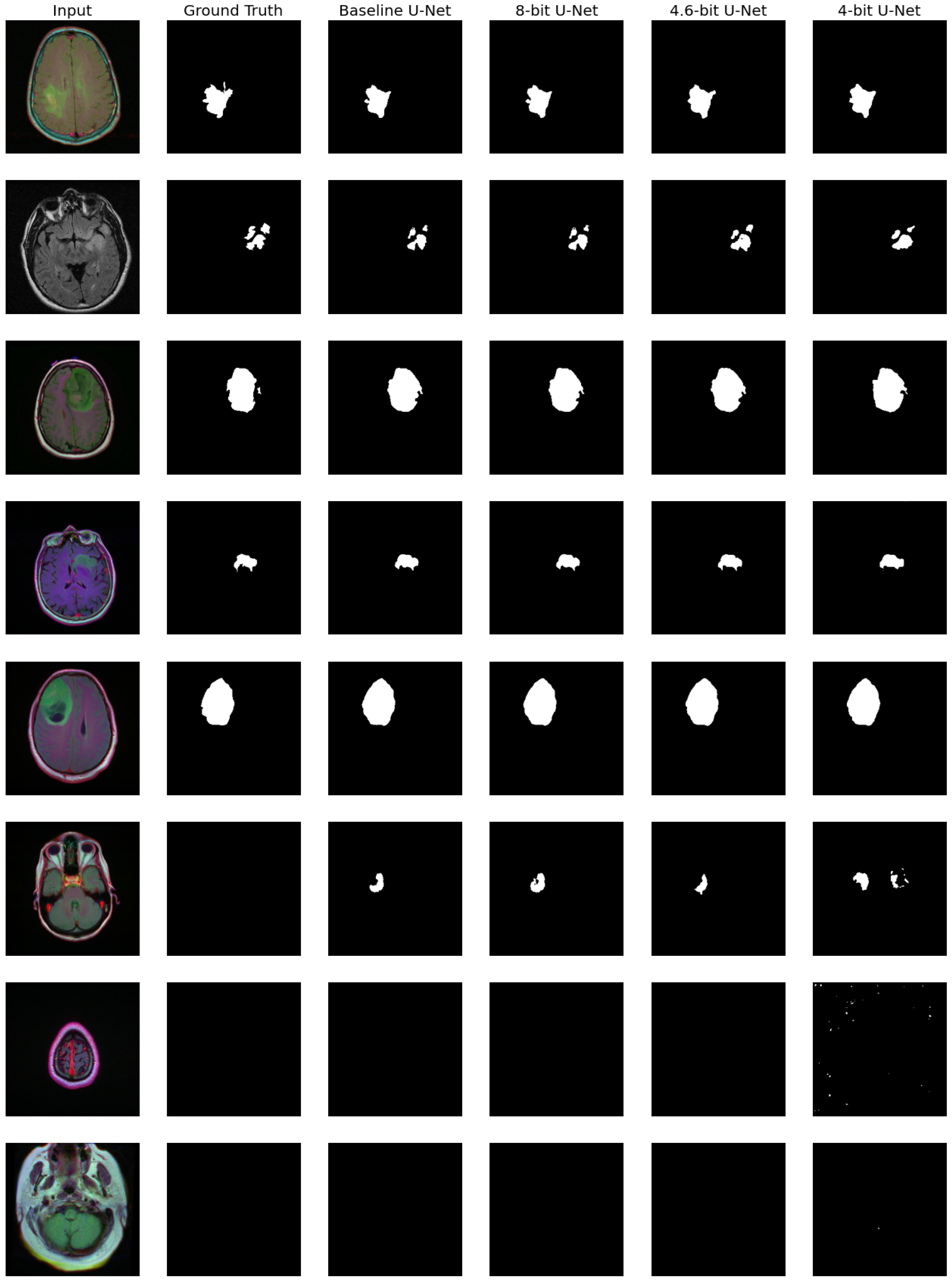
Let us now consider the U-Net model [
45]. It inputs RGB MRI images and predicts abnormality regions as binary masks. Some examples of such inputs and outputs are presented in
Figure 6.
We also computed several metrics to evaluate the resulting quality. We used Dice and Intersection over Union (IoU) scores to calculate segmentation accuracy (averaged over images at which abnormality exists). We also considered binary classification metrics (is there abnormality or not): accuracy, precision, recall, type I errors (false positive), and type II errors (false negatives). All those metrics are presented in
Table 8.
From
Figure 6 and
Table 8, we can see that eight-bit quantization is slightly better than the baseline: it increases type I error but, to some degree, improves the segmentation results. However, four-bit quantization leads to severe quality degradation and noticeable noise-like artifacts in
Figure 6. At the same time, 4.6-bit quantization preserves reasonable quality, comparable to eight-bit and baseline.
Consequently, our time measurements and training experiments prove that the proposed 4.6-bit quantization scheme can be a step between eight-bit and low-precision QNNs. It provides higher quality than four-bit quantization, working almost as fast and significantly faster than eight-bit quantization.
6. Discussion
In this paper, we proposed a 4.6-bit quantization scheme and an associated quantized matrix multiplication algorithm for fast inference of 4.6-bit quantized layers on CPUs. This matrix multiplication algorithm is very similar to that of four-bit networks but does not have the strict limitation on the depth of multiplication. That property is achieved using a loop-splitting trick, which is described at the end of
Section 4.1 and presented in Algorithm 1. If not for this trick, four- and 4.6-bit matrix multiplications would have been the same up to the data type (signed integers in 4.6-bit quantization and unsigned in four-bit quantization); thus, their computational performance would have been identical.
Since 4.6-bit quantization allows for more quantization bins than the four-bit variant, higher accuracy can be expected. Our experiment results confirmed this expectation. However, we used a relatively simple algorithm for QNN training, which can be seen as a limitation of our research. Still, even if a more advanced training method is employed and the QNN quality is higher, the 4.6-bit quantization will not be worse than the four-bit quantization because it provides more quantization bins than the four-bit one. Therefore, we can consider 4.6-bit quantization as an in-place replacement for four-bit quantization with potentially higher quality and almost the same efficiency on CPUs.
Currently, eight-bit quantization is the standard for fast neural network inference. That is why it is reasonable to compare our method with eight-bit quantization in terms of accuracy and speed. Our experiments proved that the proposed 4.6-bit quantization allows for a significant speed-up compared with eight-bit and full-precision QNNs. It works particularly well for rather large neural networks, such as ResNet-18 or ResNet-34, achieving over 40% acceleration compared with full-precision models (or over 30% compared to 8-bit counterparts).
A significant limitation of 4.6-bit quantization is the potential accuracy degradation caused by quantization. Even though it is not as high as for four-bit QNNs, it is not negligible as in eight-bit ones. However, if we consider a more complex 4.6-bit network and a simpler eight-bit network, which have the same runtime, it may turn out that the 4.6-bit network is even more accurate. Our experiments support this claim: if we compare 4.6-bit CNN8, to eight-bit CNN7 (see
Table 5 and
Table 6), we can see that the first network works faster and achieves higher accuracy than the second one. The same holds for 4.6-bit CNN9 and eight-bit CNN8. That is why we believe that our 4.6-bit quantization can serve as a useful tool when the trade-off between the quality and running time of a neural network needs to be biased towards faster computation (e.g., in real-time applications on edge devices).
It is important to note, that in our implementation of 4.6-bit multiplication, the 4.6-bit quantized values are packed into eight-bit registers, resulting in some memory overhead. However, this overhead only exists in the RAM during the computation time. In the secondary memory, the network weights can be stored using data compression techniques, achieving a memory usage of fewer than five bits per weight. When a network is initialized in RAM, those weights are decompressed back to eight-bit registers. Thus, 4.6-bit quantization can also improve secondary memory consumption, which is important for mobile devices.
4.6-bit quantization is in fact a parametric family of algorithms with different numbers of quantization bins for inputs () and weights (). In our experiments, we used the same values of those parameters for all the layers of a network. We concluded that the best results are provided by close-to-uniform distributions of bitwidth between activation and weights from , , to the symmetric , . Therefore, in practice, we can apply and expect reasonably good results. However, the ability to choose the balance of and also provides us with the opportunity to control the trade-off between network size in secondary memory (the lower the , the lower the effective bitwidth of the weights) and its quality. That may be important for some practical applications.
Let us now consider the limitations of the study. The main limitation is that we used only simple QAT and PTQ algorithms in our experiments, so they do not demonstrate the full potential of 4.6-bit quantization in terms of quality. However, our experiments prove the proposed scheme is viable and works better than four-bit quantization.
Also, in our study, we only experimented with equal quantization schemes and for all 4.6-bit quantized layers of the neural network. However, networks with mixed precision can provide the optimal balance between recognition quality and computational efficiency. Exploring 4.6-bit quantization in mixed-precision QNNs is one of the possible directions for future research. Other directions include but are not limited to the following:
Investigating more advanced techniques for 4.6-bit QNN training;
Applying 4.6-bit quantization to a wider variety of neural network architectures and different practical tasks;
And analyzing the impact of replacing eight-bit QNNs with 4.6-bit QNNs on complex recognition systems’ quality and computational efficiency.
7. Conclusions
Currently, eight-bit quantization is a standard solution for fast neural network computations on CPUs. This quantization scheme is supported by popular PyTorch and TensorFlow frameworks for both training and execution. The success of this method lies in its simplicity and efficiency for modern processor architectures, while still maintaining a high result quality.
We propose a 4.6-bit quantization scheme, which is based on the architectural features of general-purpose CPUs. This scheme minimizes the number of necessary instructions in matrix multiplication while maintaining the maximum possible number of quantization bins. So, it is an elegant and efficient expansion of the eight-bit approach. Due to the increased bitwidth for weights and activations, 4.6-bit quantization achieves higher quality than four-bit quantization while maintaining comparable speed. Therefore, it can be used as an in-place replacement for four-bit quantization with higher accuracy, or as a faster alternative for eight-bit quantization.
We experimentally evaluated the proposed scheme using various convolutional neural networks on the CIFAR-10 and ImageNet image classification datasets. The accuracy of 4.6-bit networks falls between four- and eight-bit networks, significantly improving the four-bit results. For example, quantized ResNet18 networks demonstrated the following accuracies on Image-Net dataset: 64.2% (4-bit), 66.1% (4.6-bit), and 68.7% (8-bit), respectively. For ResNet34, those accuracies are as follows: 66.1% (4-bit), 69.1% (4.6-bit), and 71.4% (8-bit). So, the accuracies of the 4.6-bit quantized model are approximately in the middle, between four-bit and eight-bit ones. However, the inference of 4.6-bit networks on CPU, which is equal to that on four-bit ones, is 1.5–1.6 times faster than that of their eight-bit counterparts.
Thus, the proposed 4.6-bit quantization is a viable scheme for fast and accurate inference of QNNs lower than eight bits on CPUs.


