Structurally Stable Astigmatic Vortex Beams with Super-High Orbital Angular Momentum (ABCD Matrix Approach)

Abstract

We have demonstrated efficiency of employing the ABCD matrix approach to transform higher-order structured Laguerre–Gaussian (sLG) beams into structurally stable astigmatic sLG (asLG) beams, highlighting their dynamics at propagating. Radical transformations of the beam structure by a cylindrical lens form not only orbital angular momentum (OAM) fast oscillations and bursts, but also make the asLG beams structurally unstable in propagation through cylindrical and spherical lenses when focusing paraxially. But, if the spherical lens performs a Fourier transform of the asLG beam after a cylindrical lens, the symmetric beam emerges at the lens focal plane with a sharp OAM dip; then, the OAM restores its former astigmatism, becoming structurally stable at the far diffraction domain. By investigating the beam structure at the focal area, we have showed that the OAM sharp dip is associated with nothing less than the process of dividing the OAM into the vortex and astigmatic constitutes predicted by Anan’ev and Bekshaev.

1. Introduction

Engineering of optical systems, based on the ABCD matrix approach developed back in the early 70s [1] of the last century (see also chapt. 20 in Ref. [2]), is the most optimal and convenient technique even now, when we have access to powerful digital software. The undoubted advantage of this approach is the ability to describe in a simple way the first-order optical system containing a cascade of conventional optical elements presented as a product of $2\times 2$ ABCD matrices M=$\left(\begin{array}{cc}A& B\\ C& D\end{array}\right)$. However, this approach works reliably only for the complex q-parameter of the fundamental Gaussian beam $1/q\left(z\right)=1/R\left(z\right)-i2/kw\left(z\right)$ containing the wavefront curvature radius $R\left(z\right)$ and the waist radius $w\left(z\right)$ of the Gaussian beam along the beam length z, where k is the wavenumber. When working with single Hermite–Gaussian (HG), Laguerre–Gaussian (LG), and other types of higher-order beams, it is already necessary to employ the Collins integral [3], written in the 2D-Kirchhoff–Fresnel approximation as [4]

$$\mathsf{\Psi }(\mathbf{r},z)=\frac{k}{2\pi iB\left(z\right)}{\int }_{{\mathbb{R}}^2}\mathsf{\Psi }\left(\rho \right)exp\left\{-i\frac{k}{2B\left(z\right)}\left[{A\left(z\right)\left|\mathit{\rho }\right|}^2-2\left(\mathit{\rho } \mathbf{r}\right)+D\left(z\right){\left|\mathbf{r}\right|}^2\right]\right\}{d}^2\mathit{\rho },$$

(1)

where $\mathsf{\Psi }\left(\mathit{\rho }\right)$ stands for a complex amplitude of the paraxial beam at the ABCD system input, $\mathit{\rho }=(\xi ,\eta )$, $\mathbf{r}=(x,y)$, $A\left(z\right)$, $B\left(z\right)$, $C\left(z\right)$, $D\left(z\right)$ are the elements of the unitary ABCD matrix with the property $AD-BC=1$.

Using this integral, Siegman [3] and later Belanger [4] gave a general outline for calculating single HG beams in a simple optical system with spherical lenses. A similar calculation for a single LG beam was carried out by Taché [5]. Alieva and Bastiaans [6,7] considered HG and HLG (Hermite–Laguerre–Gaussian) beams in first-order optical systems with a cascade of a lens, a magnifier, and an orthosymplectic system (a system that is both simplistic and orthogonal) and employed a $4\times 4$ ABCD matrix approach. Abramochkin et al. in Ref. [8] highlight key features of the ABCD approach for a general astigmatism and implemented it for HLG; Beijersbergen [9] as well as Padgett and Courtial [10] did the same for vortex mode convertors. However, if there are astigmatic elements in the optical system (i.e., cylindrical lenses), its analysis becomes significantly more complicated. Now, any cylindrical beam has to be represented in the HG mode basis whose horizontal and vertical axes are aligned with the axes of the astigmatic axes of the cylindrical lens with corresponding coordinate scaling [8,11,12,13].

The situation becomes much more complicated when using the ABCD approach for structured beams [14,15,16,17,18], which are now widely used in various fields of science and technology and which require convenient mathematical approaches for engineering optical systems. First of all, this is due to the fact that in the simplest case, it is required to represent a single LG beam in terms of HG modes in the eigen coordinate system of a cylindrical lens. It looks like this [11]

$$L{G}_{n,\pm \ell }\left(\mathbf{r}\right)=\frac{{(-1)}^n}{2^{2n+3\ell /2}n!}\sum _{k=0}^{2n+\ell }{(\pm 2\mathit{i})}^k{P}_k^{(n+\ell -k,n-k)}\left(0\right)H{G}_{2n+\ell -k,k}\left(\mathbf{r}\right),$$

(2)

here, $\mathbf{r}=(x,y)$ is a 2D vector, $P_k^{(n+\ell -k,n-k)}(.)$ is a Jacobi polynomial, and n and $\pm \ell$ are radial and azimuthal numbers of the LG beam. If the HG beam axes are rotated by an angel $\pi /4$ to the axis of the lens astigmatism, then you have to use the decomposition of the form

$$H{G}_{n,n+\ell }\left(\frac{x+y}{\sqrt{2}},\frac{x-y}{\sqrt{2}}\right)=\frac{{(-1)}^n}{2^{2n+3\ell /2}n!}\sum _{k=0}^{2n+\ell }{2}^k{P}_k^{(n+\ell -k,n-k)}\left(0\right)H{G}_{2n+\ell -k,k}\left(\mathbf{r}\right).$$

(3)

In the more complex case of arbitrary orientation of the HG beam axes relative to the lens axes, it is necessary to use the cumbersome basis transformations obtained by Alieva and Bastiaans [19]. The development of an optical system with a single astigmatic transformation of structured beams requires applications of such basic transforms to each mode of the beam, and at the same time, it is necessary to closely monitor the amplitudes and phases of the modes resulting from the transformations. When referring to the optical system that contains a sequence of astigmatic elements with different axes orientations, the basic transforms should be used for each element. As a result, the main approach to the astigmatic transformations of structured beams was focused on analyzing trajectories on the 2D sphere using the unitarity of astigmatic integral transforms [8,20,21]. On the other hand, astigmatic structured LG (sLG) beams acquire such unique properties as fast oscillations of the orbital angular momentum (OAM) when changing their control parameters [20] or shaping super-bursts of the OAM exceeding the sum of the radial and azimuthal numbers [22]. However, these properties manifest themselves only in the vicinity of the double focus of a cylindrical lens, while displacement from this plane leads to smoothing of these effects. At the same time, it is known that the OAM in the astigmatic singular beam arises due to a combination of vortex and astigmatic constitutes, the ratio of which can be controlled [13,23,24]. But this requires employing a complex optical system for which calculation of the astigmatic beam states on a 2D sphere turns out to be very cumbersome and not optimal even for computer simulation. Thus, for the instrumental implementation of the devices that transform the unstable astigmatic structured beams into structurally stable ones without losing their unique properties, engineering based on ABCD matrix technique is required.

One cannot help but remark that astigmatic processes accompany almost all optical measurements, unexpectedly manifesting themselves in light reflections and refractions on surfaces [25] or inaccurate alignment of spherical lenses [26] or cylindrical lense [26], which at once leads to distortion of the OAM laser beam. The variety of measuring techniques of these distortions is striking, ranging from standard approaches [27] and tomographic methods with mapping the distortion process onto the Poincare sphere [28] up to involving the machine learning [29]. But, on the other hand, the resulting distortions provide a unique opportunity for a simple OAM control [30], measuring the topological charge of a structured beam [31,32], as well as shaping super OAM bursts [21].

Here, we will discuss one astigmatic system that is most important for practical engineering. The system contains a cylindrical lens that forms OAM bursts and a correcting spherical lens that allows separating the astigmatic and vortex components of the OAM; it also converts a structurally unstable beam into a stable one without losing its unique properties.

2. ABCD Rule for Structured LG Beams (a Simple Astigmatism)

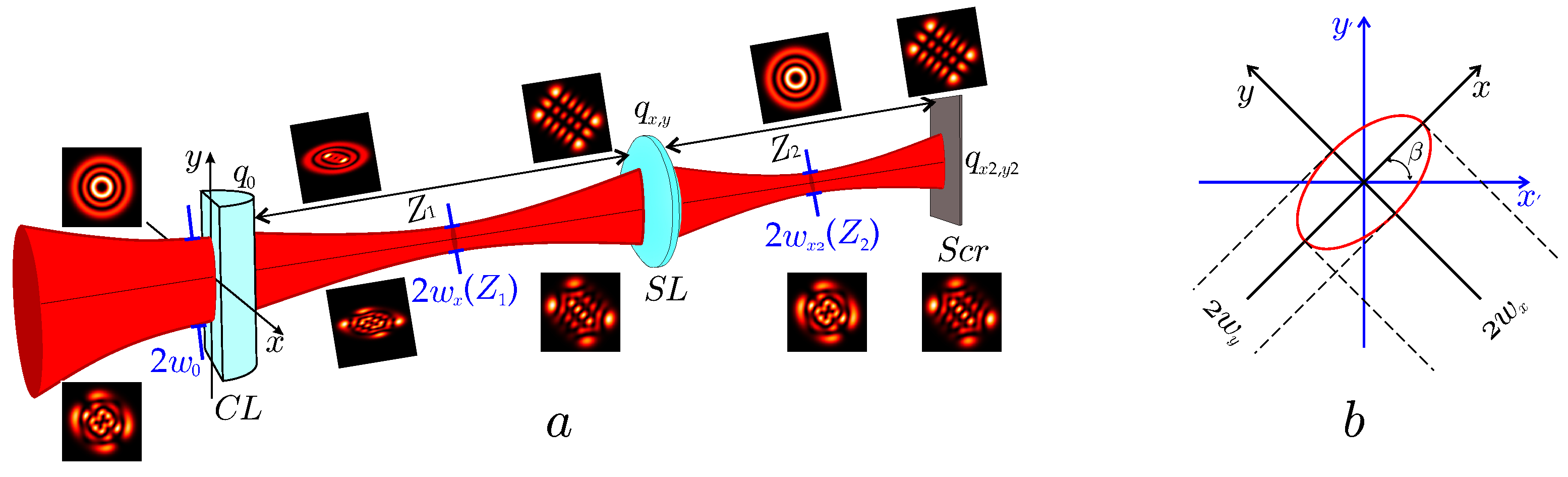
The main purpose of this section is to retrieve the optimal conditions for preserving the shape of the super OAM bursts and fast oscillations, highlighting the contribution of the beam radial number n when propagating a structured LG (sLG) beam through a cylindrical lens and separating the vortex and astigmatic OAM constitutes with a correcting spherical lens. A sketch of the optical system is shown in Figure 1a. We assume that a structured $sL{G}_{n,\ell }$ beam [33] with radial n, azimuthal ℓ numbers, and a complex parameter $q\left(z\right)=z-i{z}_0$ (where $z_0=k{w}_0/2$ is a Rayleigh length) falls onto the cylindrical lens with the focal length $f_x$ located at $z=0$ so that the initial complex parameter is $q_0=-iz$ and has a Gaussian beam waist radius of $w_0$. The spherical lens performs a Fourier transform and allows for not only separation of the vortex and astigmatic OAM constitutes, but also for transforming a structurally unstable beam into a structurally stable one without losing the OAM super-burst due to variations in the optical system parameters. In general, it is convenient to represent a complex optical system as a product of the matrices of each optical element [2]. However, since the transformation of sLG beams by astigmatic elements has not been considered before, we will first consider in detail the transformation of the sLG beam by a single cylindrical lens, determining its complex parameters $q_x$ and $q_y$. Then, we will employ them when propagating the beam through the remaining optical elements.

In fact, our inherent task is to simplify the calculation of complex optical systems of the first kind, including astigmatic elements, to make mathematics visual in comparison with the integral transformations technique (see Refs. [20,21]) and to allow for relatively simple for engineering. The best approach here, in our opinion, is a standard matrix formalism, presented below.

2.1. The Beam Structure after a Single Cylindrical Lens

We emphasize that a cylindrical lens introduces a different scale along its eigen coordinates $(x,y)$ (see Figure 1b). We assume that the axes of the cylindrical lens $(x,y)$ and the laboratory coordinates $(x^{\prime },y^{\prime })$ coincide, which corresponds to the so-called case of a simple astigmatism [8,11]. Since the HG beams are eigenmodes of an astigmatic element, we represent a sLG beam in terms of HG modes in Equation (2) but with a different scale along the coordinates $(x,y)$

$$\begin{array}{cc}\hfill & sL{G}_{n,\pm \ell }(\mathbf{r},z_1)=\frac{{(-1)}^n}{2^{2n+3\ell /2}n!}{\sum }_{j=0}^{2n+\ell }{(\pm 2i)}^j{Q}_j(1+\epsilon e^{ij\theta })P_j^{(n+\ell -j,n-j)}\left(0\right)\times \hfill \\ \hfill & \times H_{2n+\ell -j}\left(\frac{\sqrt{2}x}{w_x\left(z_1\right)}\right)H_j\left(\frac{\sqrt{2}y}{w_y\left(z_1\right)}\right)exp\left[\frac{ik}{2}\left(\frac{x^2}{q_x\left(z_1\right)}+\frac{y^2}{q_y\left(z_1\right)}\right)\right],\hfill \end{array}$$

(4)

where $H_n\left(\sqrt{2}x\right)$ is a Hermite polynomial; $Q_j$ stands for an amplitude factor, HG modes, that is written in terms of the ABCD rule as [2]:

$$Q_{x,y}={\left(\sqrt{\frac{q_{0,x,y}}{A_{x,y}·q_{0,x,y}+B_{x,y}}}\right)}^n.$$

(5)

Obviously, in the general case, we will have to use two groups of the ABCD matrices for the x and y directions, as it is written in (5)

$$q_x=\frac{A_x{q}_0(z_1=0)+B_x}{C_x{q}_0(z_1=0)+D_x},q_y=\frac{A_y{q}_0(z_1=0)+B_y}{C_y{q}_0(z_1=0)+D_y}.$$

(6)

However, the cylindrical lens does not change the scale in the y direction, so in the range $(0,z_1)$, we can write

$$q_y\left(z_1\right)=z_1-i{z}_0.$$

(7)

In the x direction, the matrix of the cylindrical lens and the displacement by the length z act as

$$M_x=\left(\begin{array}{cc}1& z_1\\ -\frac{1}{f_x}& 1\end{array}\right).$$

(8)

Then, from Equation (7), we obtain the complex parameter

$$q_x\left(z\right)=z_0\frac{\left[Z_1({\kappa }_x^2+1)-{\kappa }_x\right]-i}{{\kappa }_x^2+1},$$

(9)

where

$$Z_1=\frac{z_1}{z_0},{\kappa }_x=\frac{z_0}{f_x}.$$

(10)

The results obtained allow us to find beam radii for the x and y directions as follows $\mathrm{Re}\left(\frac{ik}{2q_x\left(z_1\right)}\right)=-\frac{1}{w_x^2\left(z_1\right)}\Rightarrow$

$$w_x^2\left(Z_1\right)=w_0^2\left[{(1-Z_1{\kappa }_x)}^2+Z_1^2\right]=w_0^2{\overline{w}}_x^2,$$

(11)

$$w_y^2\left(Z_1\right)=w_0^2(1+Z_1^2)=w_0^2{\overline{w}}_y^2,$$

(12)

as well as the mode phases

$${\mathsf{\Gamma }}_x\left(Z_1\right)=arg\sqrt{\frac{q_x}{A·q_x+B}}=\frac{1}{2}arg(1-{\kappa }_x{Z}_1+i{Z}_1),$$

(13)

$${\mathsf{\Gamma }}_y\left(Z_1\right)=\frac{1}{2}arg(1+i{Z}_1).$$

(14)

Thus, the complex amplitude of the astigmatic sLG (asLG) beam after the cylindrical lens is obtained in the form

$$\begin{array}{cc}\hfill & {\mathrm{asLG}}_{n,\ell }(x,y,Z_1|\epsilon ,\theta )=\frac{1}{\sqrt{w_x\left(Z_1\right)w_y\left(Z_1\right)}}exp\left\{-i\left[\left(2n+\ell +1/2\right){\mathsf{\Gamma }}_x\left(Z_1\right)+{\mathsf{\Gamma }}_y\left(Z_1\right)\right]\right\}\times \hfill \\ \hfill & \times \frac{{(-1)}^n}{2^{2n+3\ell /2}n!}{\sum }_{j=0}^{2n+\ell }{\left(2i\right)}^j{P}_j^{(n+\ell -j,n-\ell )}\left(0\right)\left(1+\epsilon e^{ij\theta }\right)H_{2n+\ell -j}\left(\frac{\sqrt{2}x}{w_x\left(Z_1\right)}\right)H_j\left(\frac{\sqrt{2}y}{w_y\left(Z_1\right)}\right)\times \hfill \\ \hfill & \times exp\left(ij{\mathsf{\Gamma }}_{xy}\left(Z_1\right)\right)exp\left(i\left[\frac{x^2}{{\overline{q}}_x\left(Z_1\right)}+\frac{y^2}{{\overline{q}}_y\left(Z_1\right)}\right]\right),\hfill \end{array}$$

(15)

where ${\mathsf{\Gamma }}_{xy}\left(Z_1\right)={\mathsf{\Gamma }}_y\left(Z_1\right)-{\mathsf{\Gamma }}_x\left(Z_1\right)$, $w_0=\sqrt{2z_0/k}$, $x\to x/w_0$, $y\to y/w_0$ and

$$\begin{array}{c}\hfill {\overline{q}}_x=\frac{\left[Z_1\left({\kappa }_x^2+1\right)-{\kappa }_x\right]-i}{{\kappa }_x^2+1},{\overline{q}}_y=Z_1-i.\end{array}$$

(16)

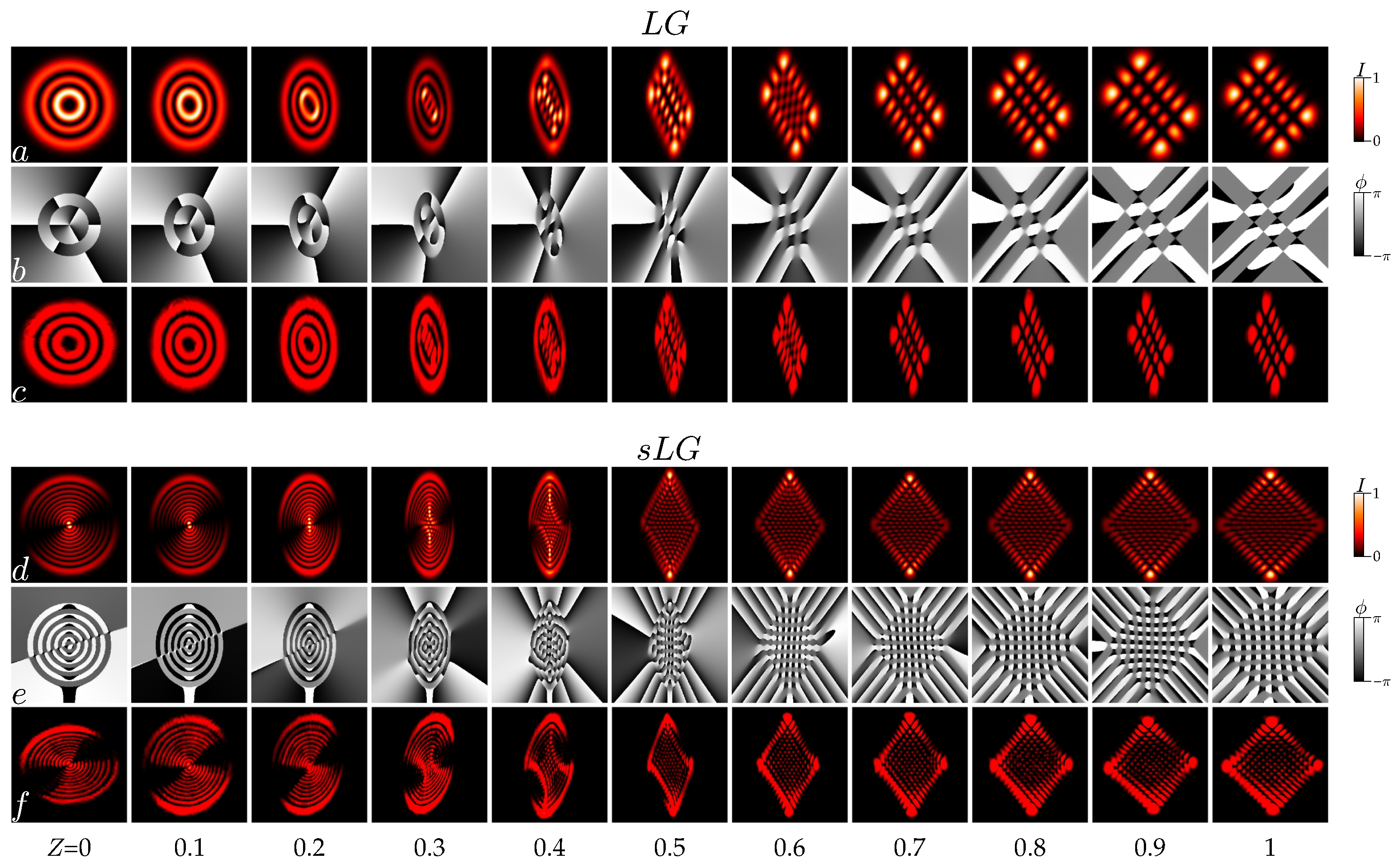
Note that the complex amplitude (15) coincides with that obtained by Baksheev et al. in Ref. [23] for the simplest case when $n=0$, $\epsilon =0$, $\theta =0$. Computer simulation (a, d) and experimental results (c, f) of the intensity and phase pattern (b, e) evolution of a single LG and structured LG beam along the propagation direction Z are illustrated in Figure 2. As expected, a single LG beam (Figure 2a–c) experiences conversion into a HG beam at length $z_1=2f_x$ ($Z_1=1$), and the number of intensity zeros along the x and y axes allows for determining the topological charge (TC) of the LG beam [34]. The intensity pattern evolution of the structured LG beam illustrates at least one interesting effect (Figure 2d–f). In the vicinity of $Z_1=1$, the intensity pattern of the asLG beam turns into an almost typical pattern of the HG mode. However, as we will show below, the beam’s OAM experiences a sharp burst. It should also be noted that the results obtained are in good agreement with the intensity patterns obtained by the method of integral transformations in Ref. [20]. However, the method of integral transformations allows us to obtain reliable results only in the far diffraction zone or in the plane of the double focus of a cylindrical lens. The expansion of the diffraction domain significantly complicates the calculation and makes the final representations of the complex amplitude very cumbersome. At the same time, the presented results based on the ABCD matrix approach significantly simplify the calculations leading to the optimal form of the complex amplitude.

2.2. The OAM Transforms

The orbital angular momentum of a structured beam, specified in the HG mode basis, is conveniently set as

$$L_z=\mathrm{Im}{\int }_{{\mathbb{R}}^2}{\mathsf{\Psi }}^{\ast }\left(\mathbf{r}\right)(x{\partial }_y-y{\partial }_x)\mathsf{\Psi }\left(\mathbf{r}\right)dxdy.$$

(17)

Obviously, the main contribution to the OAM is made by the mode amplitudes, which we find from expression (15) in the form

$$c_j={\left(2i\right)}^j{P}_j^{(n+\ell -j,n-\ell )}\left(0\right)(1+\epsilon e^{ij\theta })exp\left(ij{\mathsf{\Gamma }}_{xy}\left(z_1\right)\right).$$

(18)

Thus, employing Equation (15) in Equarion (17) we obtain

$$L_z=2^{2n+\ell }\pi \sum _{j=0}^{2n+\ell -1}(j+1)!(2n+\ell -j)!\mathrm{Im}\left(c_{j+1}{c}_j^{\ast }\right).$$

(19)

To find the OAM per photon, we calculate the energy flow along the beam z-propagation direction

$$S_z={\int }_{{\mathbb{R}}^2}\mathsf{\Psi }\left(\mathbf{r}\right){\mathsf{\Psi }}^{\ast }\left(\mathbf{r}\right)dxdy,$$

(20)

where, using Equation (18), we obtain

$$S_z=2^{2n+\ell -1}\pi \sum _{j=0}^{2n+\ell }j!(2n+\ell -j)!c_j{c}_j^{\ast }.$$

(21)

Thus, the OAM per photon is specified as

$${\ell }_z=L_z/S_z.$$

(22)

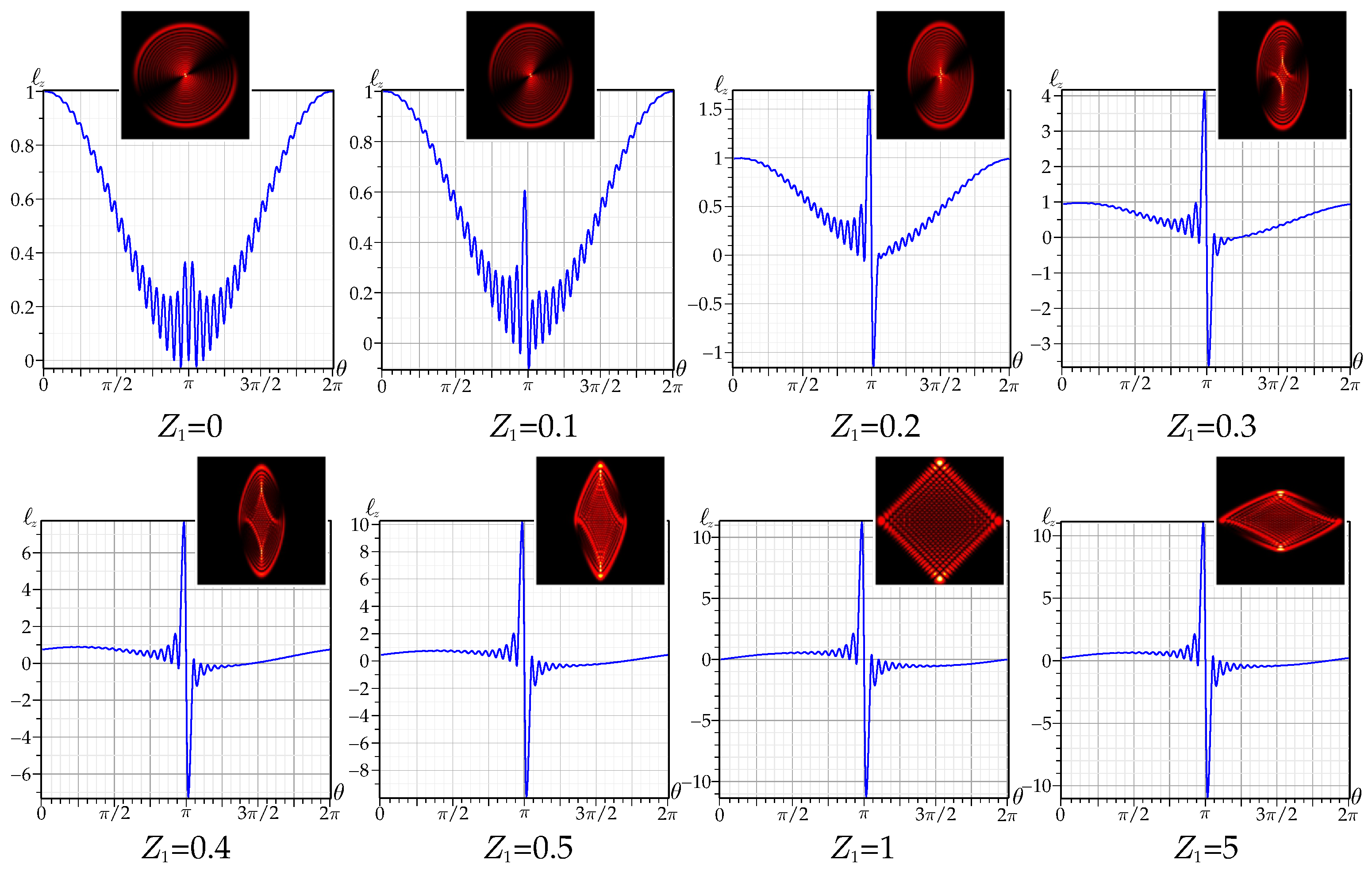
Our calculation showed that the expressions obtained can be reduced to the expression (9) obtained by Kotlyar et al. in Ref. [35], despite the fact that in their calculations, the scaling of a complex amplitude is the same along the x- and y-axes. The obtained results for the OAM ${\ell }_z\left(\theta \right)$ in Equation (22) are presented in Figure 3 in the form of fast oscillations of the OAM with variation of the control parameter $\theta$ in different cross sections $Z_1$ of the asLG beam. We see the emergence and suppression of the fast OAM oscillations as $Z_1$ shifts along the beam, while a super OAM burst is nucleating and growing near $\theta \approx 0.98\pi$. The second OAM burst with the opposite sign ${\ell }_z<0$ is brought to light at $\theta \approx 1.02\pi$. 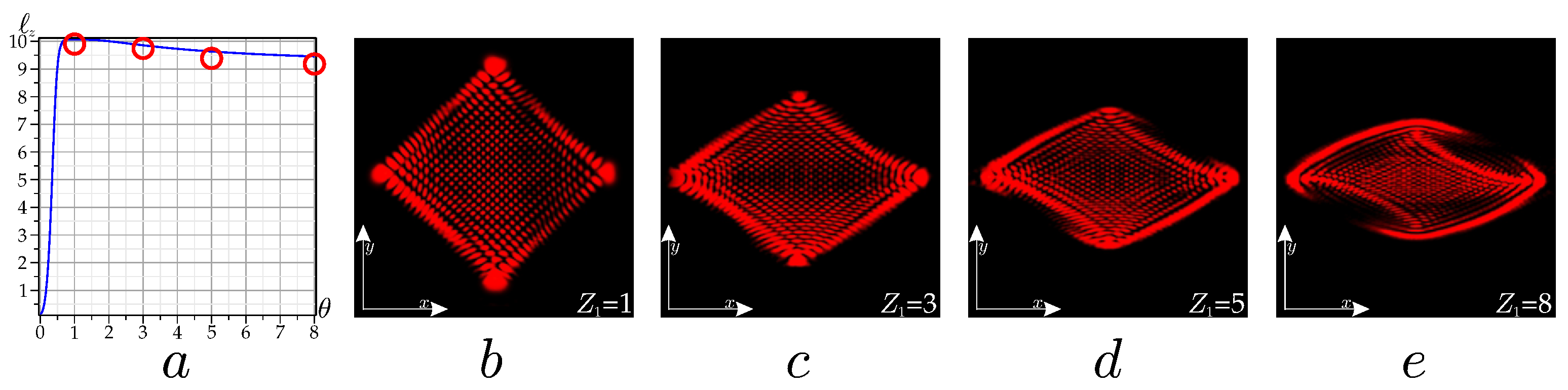Note that the OAM at $Z_1=1$ is in good agreement with the results of our paper [20] using the method of integral transformations, but the ABCD matrix technique allows us to trace the origin and evolution of fast oscillations and OAM bursts along the entire length $Z_1$ of the beam. We also see that the OAM bursts change slightly in the further diffraction zone. This keeping of the OAM burst maximum is vividly illustrated in Figure 4a. The OAM reaches its maximum value ${\ell }_z\approx 11$ at $Z_1=1$, despite the fact that the beam intensity pattern is significantly deformed (see Figure 4b–d), while the OAM tends to a half radial number ${\ell }_z\to n/2$ at the far diffraction domain.

2.3. Cylindrical and Correcting Spherical Lens

Back in the early 1990s, Anan’ev and Bekshaev showed in Ref. [36] that a singular beam OAM has astigmatic and vortex constitutes, which can be separated by means of a conventional spherical lens at the plane where the beam radii along the x and y directions become the same: $w_x\left(z\right)=w_y\left(z\right)$. Their analysis was based on the intensity moments technique of the second order. In the future, this approach was implemented for the analysis of both simple [13,23] and structured singular beams [24]. In this section, we will not delve into the math of intensity moments, but simply analyze the conditions for separating the vortex and astigmatic constitutes based on the ABCD matrix approach.

First of all, in order for a spherical lens to be a phase corrector of the asLG beam after a cylindrical lens, it must perform a Fourier transform, i.e., the transformed beam field must be located in the plane of the rear focus $f_{sh}$ of the lens, as shown in Figure 1. For the calculation, we employ the matrix (8), where the replacement is carried out $f_x⟶f_{sh}$, $z⟶z_2$. Then, the complex parameter of the beam is determined by the recurrent formula for the x direction

$$q_{x2}=\frac{z_0{\overline{q}}_x}{-\frac{z_0}{f_{sh}}{\overline{q}}_x+1}+z_0{Z}_2=z_0{\overline{q}}_{x2},$$

(23)

where

$${\overline{q}}_x=\frac{1+i\left[Z_1+{\kappa }_x\left(-1+Z_1{\kappa }_x\right)\right]}{1+{\kappa }_x^2},{\overline{q}}_{x2}=\frac{{\overline{q}}_x+Z_2\left[-{\kappa }_{sh}{\overline{q}}_x+1\right]}{1-{\kappa }_{sh}{\overline{q}}_x},$$

(24)

and ${\kappa }_{sh}=\frac{z_0}{f_{sh}}$, $Z_2=\frac{z_2}{z_0}$. We will find the x-waist radius $w_x$ of the asLG beam as

$$\frac{1}{w_{x2}^2}=-\mathrm{Re}\left(\frac{ik}{2q_{x2}}\right)=-\frac{1}{w_0^2}\mathrm{Re}\left(\frac{i}{q_{x2}}\right).$$

(25)

The beam x-phase is determined by analogy with Equation (13)

$${\mathsf{\Gamma }}_{x2}=arg\sqrt{\frac{1}{{\overline{q}}_{x2}}}.$$

(26)

The transformation of the beam x-direction by a spherical lens gives a complex parameter in the form

$$q_{y2}=z_0\frac{\left(1-Z_2{\kappa }_{sh}\right)\left(Z_1-i\right)+Z_2}{1+i{\kappa }_{sh}\left(i{Z}_1+1\right)}=z_0{\overline{q}}_{y2},$$

(27)

from where the y-waist radius and y-phase of the beam are

$$\frac{1}{w_{y2}^2}=-\mathrm{Re}\left(\frac{ik}{2q_{y2}}\right)=-\frac{1}{w_0^2}\mathrm{Re}\left(\frac{i}{{\overline{q}}_{y2}}\right),$$

(28)

$${\mathsf{\Gamma }}_{y2}=arg\left(\frac{1}{\sqrt{q_{y2}}}\right).$$

(29)

Now, the complex amplitude of the beam takes the form

$$\begin{array}{cc}\hfill & {\mathrm{asLG}}_{n,\ell }\left(x,y,z|\epsilon ,\theta \right)=\frac{1}{\sqrt{w_{x2}\left(z\right)w_{y2}\left(z\right)}}exp\left\{-i\left[\left(2n+\ell +1/2\right){\mathsf{\Gamma }}_x\left(z\right)/2+\mathsf{\Gamma }\left(z\right)/2\right]\right\}\times \hfill \\ \hfill & \times \frac{{(-1)}^n}{2^{2n+3\ell /2}n!}{\sum }_{j=0}^{2n+\ell }{\left(2i\right)}^j{P}_j^{(n+\ell -j,n-j)}\left(0\right)\left(1+\epsilon e^{ij\theta }\right)exp\left(ij{\mathsf{\Gamma }}_{k2}\left(z\right)\right)\times \hfill \\ \hfill & \times H_{2n+\ell -j}\left(\frac{\sqrt{2}x}{{\overline{w}}_{x2}\left(z\right)}\right)H_j\left(\frac{\sqrt{2}y}{{\overline{w}}_{y2}\left(z\right)}\right)exp\left(i\left[\frac{x^2}{{\overline{q}}_{x2}\left(z\right)}+\frac{y^2}{{\overline{q}}_{y2}\left(z\right)}\right]\right),\hfill \end{array}$$

(30)

where ${\mathsf{\Gamma }}_{k2}={\mathsf{\Gamma }}_{x2}-{\mathsf{\Gamma }}_{y2}$.

The curves in Figure 5 define the conditions under which the separation of the vortex and astigmatic OAM constitutes occur, as well as the transformation of a structurally unstable asLG beam into a stable one. The curves (a, d) set the conditions $w_x(Z_1,Z_2)=w_y(Z_1,Z_2)$ when the astigmatic OAM component disappears and only the vortex component makes the main contribution to the OAM [36]. It can be shown that these conditions hold for any ratio between the focal lengths of cylindrical $f_x$ and spherical $f_{sh}$ lenses. However, this does not mean that the asLG beam becomes structurally stable after the spherical lens. Two additional conditions still need to be met. The first of them requires that the difference between the radii along the x- and y-directions remain unchanged $w_x\left(Z_1,Z_2\right)-w_y\left(Z_1,Z_2\right)=const$, as shown in Figure 5b,e. This requirement imposes a restriction on the immutability of the astigmatic component during propagation after a spherical lens (see Figure 5c,f). For example, the structural stability conditions are met for all beams with parameters in Figure 5a–c at $Z_2\gg 1$. However, structurally stable handles with the parameters specified in Figure 5d–f do not tolerate OAM super-burst (see also Figure 6 and Figure 7). The second additional condition is the requirement for the spherical lens position:

$$Z_1=2f_x+f_{sh},$$

(31)

which is fulfilled for the curves in Figure 5f. Now let us look at how the OAM burst transforms after the corrective lens.

2.4. OAM after a Correcting Spherical Lens

In order to calculate the OAM, we make use of the above approach. To do this, it is sufficient to write out the amplitudes of the HG modes from Equation (30) in the form

$$c_j={\left(2i\right)}^j{p}_j^{(n+\ell -j,n-j)}\left(0\right)\left(1+\epsilon e^{ij\theta }\right)exp\left(ij{\mathsf{\Gamma }}_{k2}\left(z\right)\right).$$

(32)

After substituting Equation (30) into Equations (17)–(22), we obtain the OAM per photon as a multiparametric function ${\ell }_z={\ell }_z\left(Z_1,Z_2,f_x,f_{sh},\epsilon ,\theta ,n,\ell \right)$. The spherical lens is located at the plane (31) to perform a Fourier transform of the asLG beam after the cylindrical lens. We will peer into special points in the dependence of the OAM ${\ell }_z\left(Z_2\right)$ on the displacement $Z_2$ along the asLG beam in a state with a small $n=4$ and large $n=20$ radial number and a minimum azimuthal number $\ell =1$. The control phase parameter $\theta$ corresponds to the OAM ${\ell }_z(Z_2,\theta )$ burst at the double focus of the cylindrical lens and unit amplitude parameter $\epsilon =1$, shown in Figure 6 and Figure 7. The OAM curve ${\ell }_z\left(Z_2\right)$ in Figure 6, surrounded by intensity patterns, has a sharp dip at the points $w_x=w_y$: (a) $Z_2=0.75,n=4,\ell =1$ and (b) $Z_2=0.75,n=20,\ell =1$ corresponding to the astigmatic beam correction condition. With a spherical lens, performing a Fourier transform of a beam with the OAM burst, which corresponds to the asLG beam at the plane of the double focus of the cylindrical lens, turns the asLG beam into a non-astigmatic sLG beam; it features the beam at the cylindrical lens input. As is known [33], the OAM maximum in a structured sLG beam cannot exceed the azimuthal number $\ell =1$, while the maximum OAM of an astigmatic asLG beam exceeds half of the radial number ${\ell }_{max}>n/2$. The width of the OAM dip depends on the length $f_{sh}$ of the spherical lens focus and quickly shrinks as the focal length decreases. Then, the OAM grows sharply to its initial value, and its magnitude does not change as the observation plane shifts along the beam. Then, the OAM increases sharply to its initial value, and its magnitude does not change as the observation plane shifts along the beam, while the intensity structure also does not change. The beam becomes structurally stable up to scale and rotation. Structural stability extends to both fast oscillations and OAM bursts. Figure 7 illustrates variations in the shape of the OAM oscillations along the beam after the spherical lens. If immediately behind the spherical lens, the shape of the OAM oscillations exactly correspond to the oscillations at the plane of the double focus of the cylindrical lens; then, in the plane of matching the x- and y-radii of the beams, the nature of the oscillations changes dramatically. The oscillations take the form of the OAM oscillations before astigmatic transformations [33]. A slight offset from this plane along the beam returns the shape of the oscillations to the original form containing the featured OAM super-burst.

It is important to note that each computer simulation of intensity patterns and the OAM were accompanied by our experiment. The experimental setup and measurement techniques are described in detail in our recent article [23]. A good agreement of the experimental results with the theory based on integral transformations and the matrix ABCD approach indicate the mutual supplementation of these approaches, which can be relatively easily implemented in the engineering of modern photonics devices.

3. Conclusions

Employing the ABCD matrix approach considered in the article has significantly simplified and expanded the mathematical description of astigmatic transformations of structured beams compared to transformations on the surface of a unit sphere [20,33]. We have demonstrated the efficiency of using ABCD matrices to transform higher-order HG modes in sLG beams. It has been shown that the astigmatic transformation leads to the occurrence of the OAM super-bursts, the amplitude of which exceeds half of the radial number of the sLG beam with a minimum azimuthal number. Moreover, in contrast to transformations on the sphere, we have demonstrated the evolution of the fine intensity structure and OAM along the entire beam length. It was shown that OAM changes slightly in the far diffraction domain of the cylindrical lens, despite the fact that the sLG beam loses its structural stability.

By investigating the transformation of the sLG beam in a system of cylindrical and spherical lenses, we not only confirmed the prediction of Anan’ev and Bekshaev about the separation of the OAM vortex and astigmatic constitutes after a spherical lens [36], but also showed that a spherical lens is able to turn a structurally unstable asLG beam into a stable one in the far diffraction domain, provided that the spherical lens performs a Fourier transform of the asLG beam in the double focus of the cylindrical lens. We found that there is a sharp OAM dip in the asLG beam, where the radii of the beams are matched along the x- and y-directions $w_x\left(Z_2\right)=w_y\left(Z_2\right)$; this corresponds to suppressing the astigmatic component of the OAM, so that the main contribution to the OAM is made by the optical vortices of the beam. The asLG beam is transformed to its original sLG beam shape before the astigmatic transformation by the cylindrical lens. A slight shift of the observation plane from this area leads to a sharp grows in the OAM. The beam becomes structurally stable up to scale and rotation, while maintaining the shape of the oscillations and OAM bursts. Experimental studies are in good agreement with our computer simulation.