New Approximation Methods Based on Fuzzy Transform for Solving SODEs: I


Abstract
:1. Introduction
2. Basic Concepts
- 1.
- is continuous with , if and if ;
- 2.
- strictly increases on , and strictly decreases on ;
- 3.
- For all , This is called the Ruspini condition.
- , for all and:
- for all .
3. FzT for Solving SODEs
3.1. Methodological Remarks to Applications of the FzT
- Construction of the fuzzy partition:
- (a)
- Specify the number n of components, and compute the step .
- (b)
- Construct the nodes , where .
- (c)
- Select the shape of basic functions. We mostly use triangular- or sinusoidal-shaped basic functions. Recall that the shape of the basic functions determines the course of , that is whether it is piecewise linear or nonlinear.
- (d)
- Construct a uniform fuzzy partition of by triangular- or sinusoidal-shaped basic functions [5].
- Computation of FzT: We replace by their approximations based on the Taylor expansion as new functions with respect to the fuzzy partition by Step 1. In this way, similarly to [6], we transfer the original SODEs to the space of fuzzy units, solve them in the new space and then transfer them back by the inverse FzT. Compute the approximation for x and y by the inverse FzT applied to and . In the next subsections, the schemes provide formulas for the computation of components of FzT.
3.2. Numerical Scheme I for SODEs
- 1.
- for a value of k in the range :where .
- 2.
- for all :where and .
- Using (6), we can get for each and :Based on Remark 1 and Definition 1, the properties of the uniform fuzzy partition, we replace t by and then by . Thus,In a similar way, .
- We first prove the estimate for . Then, we show that for all , by using Lemma 2, for ,where . By (15), we get:By using (25), we get:where , and . In particular,where we have used inequality . Analogously, . which concludes the proof.
- Case 1.
- If , , we get:where . Indeed, we have used inequality , , and the quantity is a finite geometric series; these can be calculated by:In particular, when , this implies that:
- Case 2.
- In view of Remark 5, let ,Thus,where and . Consequently,where . In particular, when , this implies that:and if a sequence of , we get , , which concludes the proof. ☐
3.3. Numerical Scheme II for SODEs
- 1.
- for a value of k in the range :where .
- 2.
- for allwhere and .
- ,
- , , ,
- , , ,
- is the upper bound of , , and .
4. Applications
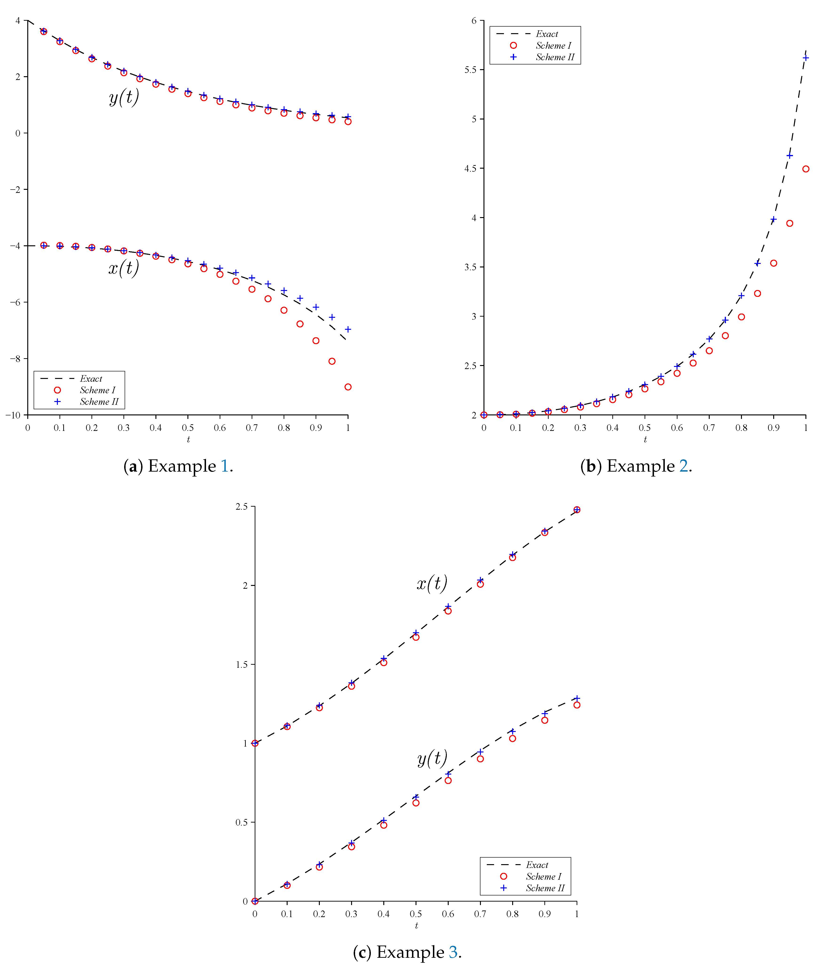
- Moreover, a comparison of MSE for Examples 1–3 is shown in Table 1. It is observed that the new fuzzy approximation methods yield more accurate results in comparison with the classical Euler and classical trapezoidal rule (one-step). The best result (in comparison with the Schemes I and II) is obtained by Scheme II.
5. Conclusions
Author Contributions
Funding
Acknowledgments
Conflicts of Interest
Appendix A. Taylor Series
Appendix B. Algorithms

| INPUT: and in Equation (5); endpoints ; integer N; initial condition . |
| Step 1 Set ; ; ; ; ; . |
| Step 2 Define the generalized uniform fuzzy partitions as . |
| Step 3 For to N, do Steps 4–7. |
| end. |
| OUTPUT: Approximation X and Y to x and y, respectively, at the () values of t. |
| INPUT: ; ; endpoints ; integer N; initial condition . |
| Step 1 Set ; ; ; ; ; . |
| Step 2 Define the generalized uniform fuzzy partitions as . |
| Step 3 For to N, do Steps 4–11. |
| end. |
| OUTPUT: Approximation X and Y to x and y, respectively, at the () values of t. |
References
- Ahmad, M.Z.; Hasan, M.K.; Baets, B.D. Analytical and numerical solutions of fuzzy differential equations. Inf. Sci. 2013, 236, 156–167. [Google Scholar] [CrossRef]
- Shawagfeh, N.; Kaya, D. Comparing numerical methods for the solutions of systems of ordinary differential equations. Appl. Math. Lett. 2004, 17, 323–328. [Google Scholar] [CrossRef]
- Atkinson, K.; Han, W.; Stewart, D. Numerical Solution of Ordinary Differential Equations; Wiley: New York, NY, USA, 2009. [Google Scholar]
- Ahmad, M.Z.; De Baets, B. A Predator-Prey Model with Fuzzy Initial Populations. In Proceedings of the Joint 13th IFSA World Congress and 6th EUSFLAT Conference, Lisbon, Portugal, 20–24 July 2009; pp. 1311–1314. [Google Scholar]
- Perfilieva, I. Fuzzy transforms: Theory and applications. Fuzzy Sets Syst. 2006, 157, 993–1023. [Google Scholar] [CrossRef]
- Perfilieva, I. Fuzzy transform: Application to the Reef growth problem. In Fuzzy Logic in Geology; Demicco, R.V., Klir, G.J., Eds.; Academic Press: Amsterdam, The Netherlands, 2003; Chapter 9; pp. 275–300. [Google Scholar]
- Perfilieva, I.; Daňková, M.; Bede, B. Towards a higher degree F-transform. Fuzzy Sets Syst. 2011, 180, 3–19. [Google Scholar] [CrossRef]
- Chen, W.; Shen, Y. Approximate solution for a class of second-order ordinary differential equations by the fuzzy transform. J. Intell. Fuzzy Syst. 2014, 27, 73–82. [Google Scholar]
- Alireza, K.; Zahra, A.; Irina, P. Fuzzy transform to approximate solution of two-point boundary value problems. Math. Meth. Appl. Sci. 2017, 40, 6147–6154. [Google Scholar]
- Tomasiello, S. An alternative use of fuzzy transform with application to a class of delay differential equations. Int. J. Comput. Math. 2017, 94, 1719–1726. [Google Scholar] [CrossRef]
- Hodakova, P.; Perfilieva, I.; Valasek, R. A new approach to fuzzy boundary value problem. In Uncertainty Modelling in Knowledge Engineering and Decision Making; World Scientific Proceedings Series on Computer Engineering and Information Science; World Scientific Publishing Company: Singapore, 2016; Volume 10, pp. 276–281. ISBN 978-981-3146-96-9. [Google Scholar]
- Perfilieva, I.; Števuliáková, P.; Valášek, R. F-transform for numerical solution of two-point boundary value problem. Iran. J. Fuzzy Syst. 2017, 14, 1–13. [Google Scholar]
- Perfilieva, I.; Števuliáková, P.; Valášek, R. F-transform-based shooting method for nonlinear boundary value problems. Soft Comput. 2017, 21, 3493–3502. [Google Scholar] [CrossRef]
- Alijani, Z.; Khastan, A.; Khattri, S.K.; Tomasiello, S. Fuzzy Transform to Approximate Solution of Boundary Value Problems via Optimal Coefficients. In Proceedings of the 2017 International Conference on High Performance Computing Simulation (HPCS), Genoa, Italy, 17–21 July 2017; pp. 466–471. [Google Scholar]
- Alikhani, R.; Zeinali, M.; Bahrami, F.; Shahmorad, S.; Perfilieva, I. Trigonometric Fm-transform and its approximative properties. Soft Comput. 2017, 21, 3567–3577. [Google Scholar] [CrossRef]
- Jahedi, S.; Javadi, F.; Mehdipour, M.J. Weighted transform and approximation of some functions on unbounded sets. Soft Comput. 2017, 21, 3579–3585. [Google Scholar] [CrossRef]
- Tomasiello, S.; Gaeta, M.; Loia, V. Quasi–consensus in Second–Order Multi–agent Systems with Sampled Data Through Fuzzy Transform. J. Uncertain Syst. 2016, 10, 243–250. [Google Scholar]
- Tomasiello, S. A First Investigation on the Dynamics of Two Delayed Neurons through Fuzzy Transform Approximation. In Proceedings of the 2017 International Conference on High Performance Computing Simulation (HPCS), Genoa, Italy, 17–21 July 2017; pp. 460–465. [Google Scholar]
- Alkasasbeh, H.A.; Perfilieva, I.; Ahmad, M.Z.; Yahya, Z.R. New fuzzy numerical methods for solving Cauchy problems. Appl. Syst. Innov. 2018, 1, 15. [Google Scholar] [CrossRef]
- Parapari, H.F.; Menhaj, M.B. Solving nonlinear ordinary differential equations using neural networks. In Proceedings of the 2016 4th International Conference on Control, Instrumentation, and Automation (ICCIA), Qazvin, Iran, 27–28 January 2016; pp. 351–355. [Google Scholar]
- Ramos, H.; Singh, G.; Kanwar, V.; Bhatia, S. An embedded 3 (2) pair of nonlinear methods for solving first order initial-value ordinary differential systems. Numer. Algorithms 2017, 75, 509–529. [Google Scholar] [CrossRef]
- Perez, J.F.S.; Conesa, M.; Alhama, I. Solving ordinary differential equations by electrical analogy: A multidisciplinary teaching tool. Eur. J. Phys. 2016, 37, 065703. [Google Scholar] [CrossRef]
- Al-Omari, A.; Arnold, J.; Taha, T.; Schüttler, H.B. Solving Large Nonlinear Systems of First-Order Ordinary Differential Equations with Hierarchical Structure Using Multi-GPGPUs and an Adaptive Runge Kutta ODE Solver. IEEE Access 2013, 1, 770–777. [Google Scholar] [CrossRef]
- Opanuga, A.; Edeki, S.; Okagbue, H.; Akinlabi, G.; Osheku, A.; Ajayi, B. On numerical solutions of systems of ordinary differential equations by numerical-analytical method. Appl. Math. Sci. 2014, 8, 8199–8207. [Google Scholar] [CrossRef]
- Al-Omari, A.; Schuttler, H.B.; Arnold, J.; Taha, T. Solving Nonlinear Systems of First Order Ordinary Differential Equations Using a Galerkin Finite Element Method. IEEE Access 2013, 1, 408–417. [Google Scholar] [CrossRef]
- Matveev, S.A.; Smirnov, A.P.; Tyrtyshnikov, E. A fast numerical method for the Cauchy problem for the Smoluchowski equation. J. Comput. Phys. 2015, 282, 23–32. [Google Scholar] [CrossRef]
- Mondal, S.P.; Roy, T.K. First order homogeneous ordinary differential equation with initial value as triangular intuitionistic fuzzy number. J. Uncertain. Math. Sci. 2014, 2014, 1–17. [Google Scholar] [CrossRef] [Green Version]
- Mondal, S.P.; Roy, T.K. System of Differential Equation with Initial Value as Triangular Intuitionistic Fuzzy Number and its Application. Int. J. Appl. Comput. Math. 2015, 1, 449–474. [Google Scholar] [CrossRef] [Green Version]
- Paul, S.; Mondal, S.P.; Bhattacharya, P. Numerical solution of Lotka Volterra prey predator model by using Runge-Kutta-Fehlberg method and Laplace Adomian decomposition method. Alex. Eng. J. 2016, 55, 613–617. [Google Scholar] [CrossRef]
- Yusufoğlu, E.; Erbaş, B. He’s variational iteration method applied to the solution of the prey and predator problem with variable coefficients. Phys. Lett. A 2008, 372, 3829–3835. [Google Scholar] [CrossRef]
- Li, J.; Zhao, A. Stability analysis of a non-autonomous Lotka-Volterra competition model with seasonal succession. Appl. Math. Modell. 2016, 40, 763–781. [Google Scholar] [CrossRef]
- Khastan, A.; Perfilieva, I.; Alijani, Z. A new fuzzy approximation method to Cauchy problems by fuzzy transform. Fuzzy Sets Syst. 2016, 288, 75–95. [Google Scholar] [CrossRef]
- Bougoffa, L. Solvability of the predator and prey system with variable coefficients and comparison of the results with modified decomposition. Appl. Math. Comput. 2006, 182, 383–387. [Google Scholar] [CrossRef]
- González-Parra, G.C.; Arenas, A.J.; Cogollo, M.R. Numerical-analytical solutions of predator-prey models. WSEAS Trans. Biol. Biomed. 2013, 10, 79–87. [Google Scholar]
- Butcher, J.C. Numerical Methods for Ordinary Differential Equations, 3rd ed.; John Wiley & Sons, Ltd.: Chichester, UK, 2016. [Google Scholar]
- Burden, R.L.; Faires, J.D. Numerical Analysis, 9th ed.; Brooks/Cole Cengage Learning: Boston, MA, USA, 2010; ISBN 978-0-538-73351-9. [Google Scholar]
- Alkasasbeh, H.A.; Perfilieva, I.; Ahmad, M.Z.; Yahya, Z.R. New approximation methods based on fuzzy transform for solving SODEs: II. Appl. Syst. Innov. 2018, 1, 30. [Google Scholar]

| Method | Example 1 | Example 2 | Example 3 | |||
|---|---|---|---|---|---|---|
| Scheme I | 2.91443 × 10 | 6.67431 × 10 | 1.12399 × 10 | 1.12399 × 10 | 2.92534 × 10 | 1.58256 × 10 |
| Scheme II | 2.24139 × 10 | 3.77476 × 10 | 3.04846 × 10 | 3.04846 × 10 | 1.72082 × 10 | 4.10161 × 10 |
| Euler | 6.99731 × 10 | 1.19826 × 10 | 1.14890 × 10 | 1.14890 × 10 | 5.43867 × 10 | 1.68059 × 10 |
| Trapezoidal | 5.99915 × 10 | 1.40165 × 10 | 2.75574 × 10 | 2.75574 × 10 | 3.19103 × 10 | 5.21595 × 10 |
| Solution | Proposed Scheme I | Proposed Scheme II | Euler | Trapezoidal | |
|---|---|---|---|---|---|
| 0.00 | 1.00000 | 1.00000 | 1.00000 | 1.00000 | 1.00000 |
| 0.10 | 1.10965 | 1.10581 | 1.11259 | 1.10000 | 1.10945 |
| 0.20 | 1.23706 | 1.22517 | 1.24000 | 1.21890 | 1.23671 |
| 0.30 | 1.37957 | 1.36112 | 1.38257 | 1.35438 | 1.37924 |
| 0.40 | 1.53406 | 1.51087 | 1.53717 | 1.50368 | 1.53402 |
| 0.50 | 1.69689 | 1.67119 | 1.70015 | 1.66355 | 1.69755 |
| 0.60 | 1.86386 | 1.83827 | 1.86733 | 1.83022 | 1.86575 |
| 0.70 | 2.03020 | 2.00777 | 2.03392 | 1.99935 | 2.03396 |
| 0.80 | 2.19055 | 2.17473 | 2.19456 | 2.16601 | 2.19692 |
| 0.90 | 2.33891 | 2.33356 | 2.34322 | 2.32461 | 2.34870 |
| 1.00 | 2.46869 | 2.47798 | 2.47776 | 2.46891 | 2.48270 |
| Solution | Proposed Scheme I | Proposed Scheme II | Euler | Trapezoidal | |
|---|---|---|---|---|---|
| 0.00 | 0.00000 | 0.00000 | 0.00000 | 0.00000 | 0.00000 |
| 0.10 | 0.10933 | 0.09948 | 0.10781 | 0.10000 | 0.10805 |
| 0.20 | 0.23466 | 0.21563 | 0.23168 | 0.21610 | 0.23113 |
| 0.30 | 0.37191 | 0.34407 | 0.36755 | 0.34440 | 0.36521 |
| 0.40 | 0.51694 | 0.48088 | 0.51126 | 0.48098 | 0.50621 |
| 0.50 | 0.66544 | 0.62209 | 0.65855 | 0.62184 | 0.64994 |
| 0.60 | 0.81285 | 0.76359 | 0.80488 | 0.76288 | 0.79202 |
| 0.70 | 0.95430 | 0.90109 | 0.94543 | 0.89979 | 0.92782 |
| 0.80 | 1.08451 | 1.03002 | 1.07494 | 1.02801 | 1.05236 |
| 0.90 | 1.19767 | 1.14549 | 1.18766 | 1.14261 | 1.16023 |
| 1.00 | 1.28736 | 1.24213 | 1.28463 | 1.23823 | 1.24549 |
| Solution | Proposed Scheme I | Proposed Scheme II | Euler | Trapezoidal | |
|---|---|---|---|---|---|
| 0.00 | −4.00000 | −4.00000 | −4.00000 | −4.00000 | −4.00000 |
| 0.05 | −4.00501 | −3.97865 | −3.99616 | −4.00000 | −4.00714 |
| 0.10 | −4.02008 | −3.99232 | −4.01193 | −4.01429 | −4.02627 |
| 0.15 | −4.04543 | −4.01914 | −4.03732 | −4.04276 | −4.05752 |
| 0.20 | −4.08136 | −4.05937 | −4.07264 | −4.08574 | −4.10134 |
| 0.25 | −4.12834 | −4.11358 | −4.11833 | −4.14389 | −4.15850 |
| 0.30 | −4.18701 | −4.18268 | −4.17490 | −4.21830 | −4.23015 |
| 0.35 | −4.25816 | −4.26794 | −4.24305 | −4.31052 | −4.31783 |
| 0.40 | −4.34282 | −4.37105 | −4.32359 | −4.42260 | −4.42361 |
| 0.45 | −4.44224 | −4.49423 | −4.41752 | −4.55722 | −4.55014 |
| 0.50 | −4.55798 | −4.64028 | −4.52605 | −4.71784 | −4.70086 |
| 0.55 | −4.69195 | −4.81278 | −4.65062 | −4.90891 | −4.88023 |
| 0.60 | −4.84651 | −5.01628 | −4.79297 | −5.13613 | −5.09399 |
| 0.65 | −5.02460 | −5.25662 | −4.95520 | −5.40685 | −5.34964 |
| 0.70 | −5.22984 | −5.54127 | −5.13983 | −5.73061 | −5.65700 |
| 0.75 | −5.46680 | −5.87990 | −5.34992 | −6.11990 | −6.02912 |
| 0.80 | −5.74130 | −6.28518 | −5.58925 | −6.59122 | −6.48349 |
| 0.85 | −6.06076 | −6.77381 | −5.86249 | −7.16663 | −7.04390 |
| 0.90 | −6.43490 | −7.36820 | −6.17551 | −7.87602 | −7.74310 |
| 0.95 | −6.87660 | −8.09874 | −6.53582 | −8.76042 | −8.62699 |
| 1.00 | −7.40326 | −9.00740 | −6.96630 | −9.87710 | −9.76103 |
| Solution | Proposed Scheme I | Proposed Scheme II | Euler | Trapezoidal | |
|---|---|---|---|---|---|
| 0.00 | 4.00000 | 4.00000 | 4.00000 | 4.00000 | 4.00000 |
| 0.05 | 3.61935 | 3.60013 | 3.62249 | 3.60000 | 3.62045 |
| 0.10 | 3.27492 | 3.24497 | 3.28040 | 3.24090 | 3.27766 |
| 0.15 | 2.96327 | 2.92506 | 2.97057 | 2.91774 | 2.96757 |
| 0.20 | 2.68128 | 2.63645 | 2.69004 | 2.62635 | 2.68671 |
| 0.25 | 2.42612 | 2.37573 | 2.43612 | 2.36315 | 2.43201 |
| 0.30 | 2.19525 | 2.13994 | 2.20634 | 2.12506 | 2.20079 |
| 0.35 | 1.98634 | 1.92646 | 1.99847 | 1.90938 | 1.99067 |
| 0.40 | 1.79732 | 1.73299 | 1.81047 | 1.71374 | 1.79951 |
| 0.45 | 1.62628 | 1.55749 | 1.64050 | 1.53607 | 1.62541 |
| 0.50 | 1.47152 | 1.39815 | 1.48689 | 1.37451 | 1.46664 |
| 0.55 | 1.33148 | 1.25333 | 1.34811 | 1.22742 | 1.32166 |
| 0.60 | 1.20478 | 1.12159 | 1.22279 | 1.09333 | 1.18908 |
| 0.65 | 1.09013 | 1.00161 | 1.10969 | 0.97093 | 1.06762 |
| 0.70 | 0.98639 | 0.89223 | 1.00768 | 0.85906 | 0.95615 |
| 0.75 | 0.89252 | 0.79241 | 0.91576 | 0.75670 | 0.85366 |
| 0.80 | 0.80759 | 0.70122 | 0.83301 | 0.66295 | 0.75923 |
| 0.85 | 0.73073 | 0.61784 | 0.75862 | 0.57703 | 0.67208 |
| 0.90 | 0.66120 | 0.54154 | 0.69184 | 0.49827 | 0.59150 |
| 0.95 | 0.59827 | 0.47170 | 0.63202 | 0.42612 | 0.51692 |
| 1.00 | 0.54134 | 0.40778 | 0.57734 | 0.36016 | 0.44787 |
| Solution | Proposed Scheme I | Proposed Scheme II | Euler | Trapezoidal | |
|---|---|---|---|---|---|
| 0.00 | 2.00000 | 2.00000 | 2.00000 | 2.00000 | 2.00000 |
| 0.05 | 2.00250 | 2.00149 | 2.00325 | 2.00000 | 2.00250 |
| 0.10 | 2.01008 | 2.00650 | 2.01082 | 2.00500 | 2.01005 |
| 0.15 | 2.02289 | 2.01660 | 2.02364 | 2.01508 | 2.02279 |
| 0.20 | 2.04124 | 2.03197 | 2.04201 | 2.03042 | 2.04101 |
| 0.25 | 2.06557 | 2.05294 | 2.06636 | 2.05134 | 2.06511 |
| 0.30 | 2.09650 | 2.07996 | 2.09731 | 2.07830 | 2.09567 |
| 0.35 | 2.13485 | 2.11365 | 2.13568 | 2.11191 | 2.13344 |
| 0.40 | 2.18171 | 2.15485 | 2.18256 | 2.15301 | 2.17942 |
| 0.45 | 2.23852 | 2.20462 | 2.23939 | 2.20265 | 2.23493 |
| 0.50 | 2.30720 | 2.26437 | 2.30808 | 2.26226 | 2.30167 |
| 0.55 | 2.39031 | 2.33595 | 2.39116 | 2.33365 | 2.38192 |
| 0.60 | 2.49133 | 2.42177 | 2.49211 | 2.41923 | 2.47868 |
| 0.65 | 2.61513 | 2.52506 | 2.61574 | 2.52224 | 2.59605 |
| 0.70 | 2.76863 | 2.65022 | 2.76888 | 2.64702 | 2.73967 |
| 0.75 | 2.96202 | 2.80329 | 2.96157 | 2.79961 | 2.91754 |
| 0.80 | 3.21093 | 2.99285 | 3.20907 | 2.98854 | 3.14130 |
| 0.85 | 3.54059 | 3.23143 | 3.53586 | 3.22625 | 3.42845 |
| 0.90 | 3.99443 | 3.53788 | 3.98346 | 3.53151 | 3.80653 |
| 0.95 | 4.65413 | 3.94192 | 4.62841 | 3.93381 | 4.32100 |
| 1.00 | 5.69348 | 4.49277 | 5.61875 | 4.48201 | 5.05197 |
| Case | Proposed Scheme for | Proposed Scheme for | |||
|---|---|---|---|---|---|
| I | II | I | II | ||
| Ex.1 | T | 2.48353 × 10 | 3.37890 × 10 | 6.03282 × 10 | 5.38734 × 10 |
| C | 2.91443 × 10 | 2.24139 × 10 | 6.67431 × 10 | 3.77476 × 10 | |
| Ex.2 | T | 1.12099 × 10 | 3.01900 × 10 | 1.12099 × 10 | 3.01900 × 10 |
| C | 1.12399 × 10 | 3.04846 × 10 | 1.12399 × 10 | 3.04846 × 10 | |
| Ex.3 | T | 2.71905 × 10 | 2.08807 × 10 | 1.61509 × 10 | 4.84176 × 10 |
| C | 2.92534 × 10 | 1.72082 × 10 | 1.58256 × 10 | 4.10161 × 10 | |
© 2018 by the authors. Licensee MDPI, Basel, Switzerland. This article is an open access article distributed under the terms and conditions of the Creative Commons Attribution (CC BY) license (http://creativecommons.org/licenses/by/4.0/).
Share and Cite
ALKasasbeh, H.; Perfilieva, I.; Ahmad, M.Z.; Yahya, Z.R. New Approximation Methods Based on Fuzzy Transform for Solving SODEs: I. Appl. Syst. Innov. 2018, 1, 29. https://doi.org/10.3390/asi1030029
ALKasasbeh H, Perfilieva I, Ahmad MZ, Yahya ZR. New Approximation Methods Based on Fuzzy Transform for Solving SODEs: I. Applied System Innovation. 2018; 1(3):29. https://doi.org/10.3390/asi1030029
Chicago/Turabian StyleALKasasbeh, Hussein, Irina Perfilieva, Muhammad Zaini Ahmad, and Zainor Ridzuan Yahya. 2018. "New Approximation Methods Based on Fuzzy Transform for Solving SODEs: I" Applied System Innovation 1, no. 3: 29. https://doi.org/10.3390/asi1030029
APA StyleALKasasbeh, H., Perfilieva, I., Ahmad, M. Z., & Yahya, Z. R. (2018). New Approximation Methods Based on Fuzzy Transform for Solving SODEs: I. Applied System Innovation, 1(3), 29. https://doi.org/10.3390/asi1030029