To keep track of the most representative trajectory points, a pre-processing step is applied. The objective behind is to eliminate noisy data due to some positioning mismatch or errors. A Kalman Filter is applied in a sort of recursive algorithm by considering a covariance matrix of a series of points. A simple linear model is applied to determine the first line of each trajectory. Therefore, the variance (σ) of the distance between two consecutive points in a given trajectory is calculated, and the points with greater distance than (2σ) from the fitting line are detected as noisy data and eliminated.
3.1. Critical Points Detection
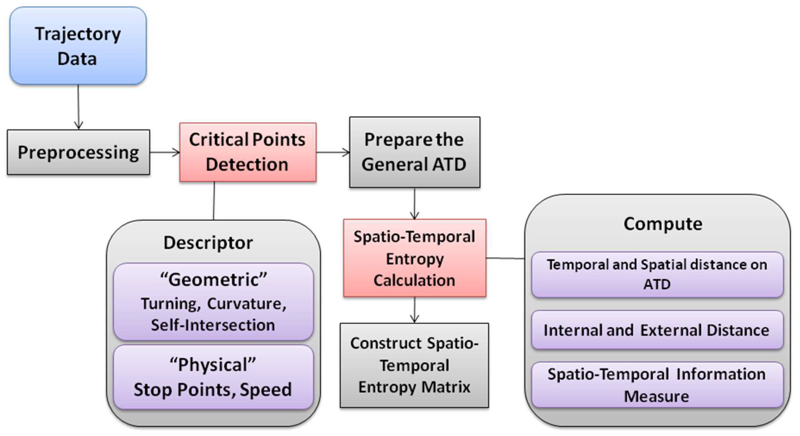
The first methodological objective is the derivation of a minimum number of critical points according to the geometric and semantic characteristics of some trajectory data. Extra trajectory data not specifically relevant and noisy will be eliminated to facilitate further processing times. The geometric parameters considered include curvature, turning and self-intersection points. They are detected by the application of a convex hull structure as introduced in our previous work [
58]. More precisely, these three geometric parameters can be defined as follows:
Curvature: a curvature denotes a curve in a trajectory and a curvature point is defined as the central point of the curve.
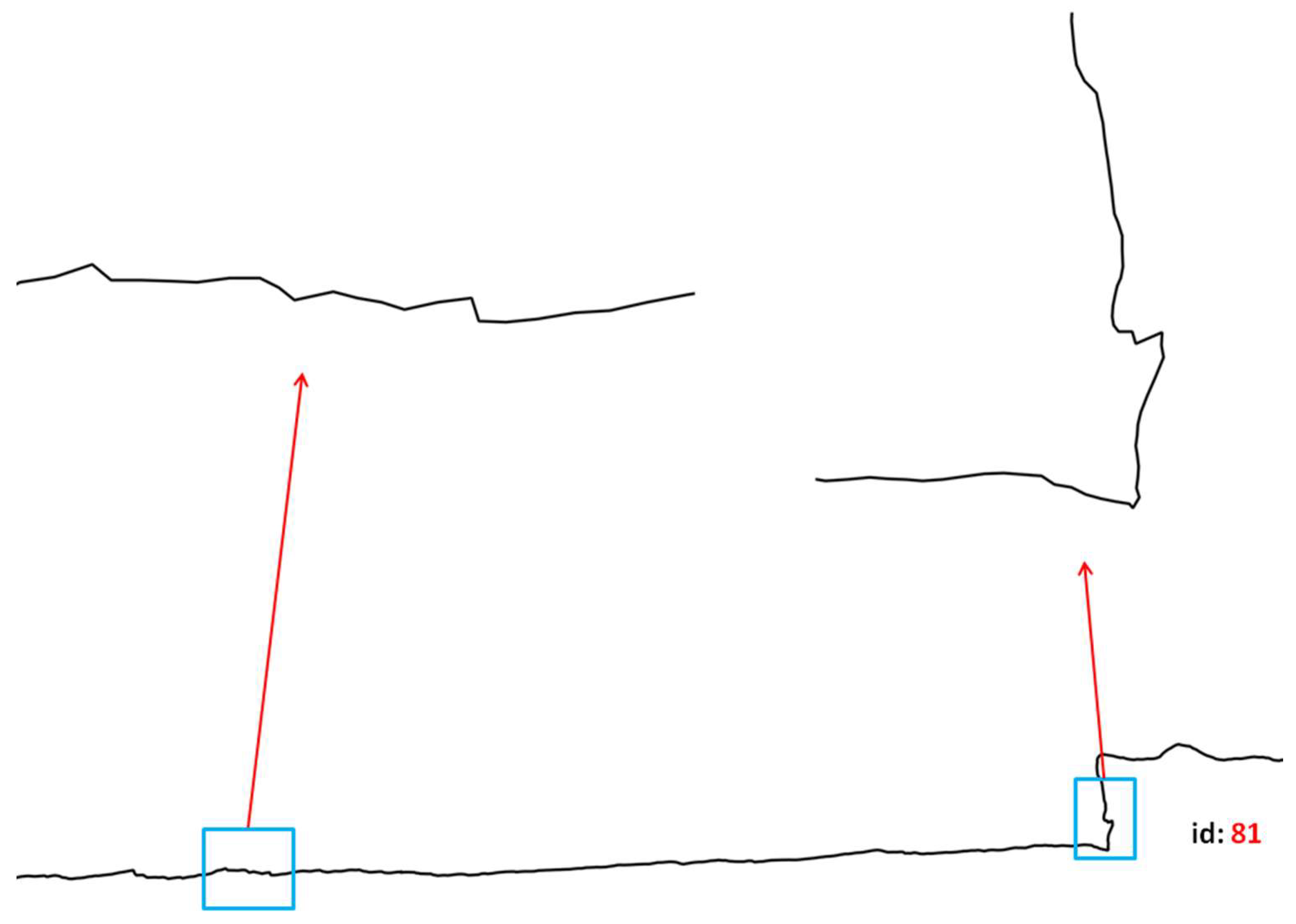
Turning point: a turning point is considered to be a changing direction point of a trajectory. For instance, a straight trajectory with no curve does not have any turning points while two turning points arise for each trajectory curvature.
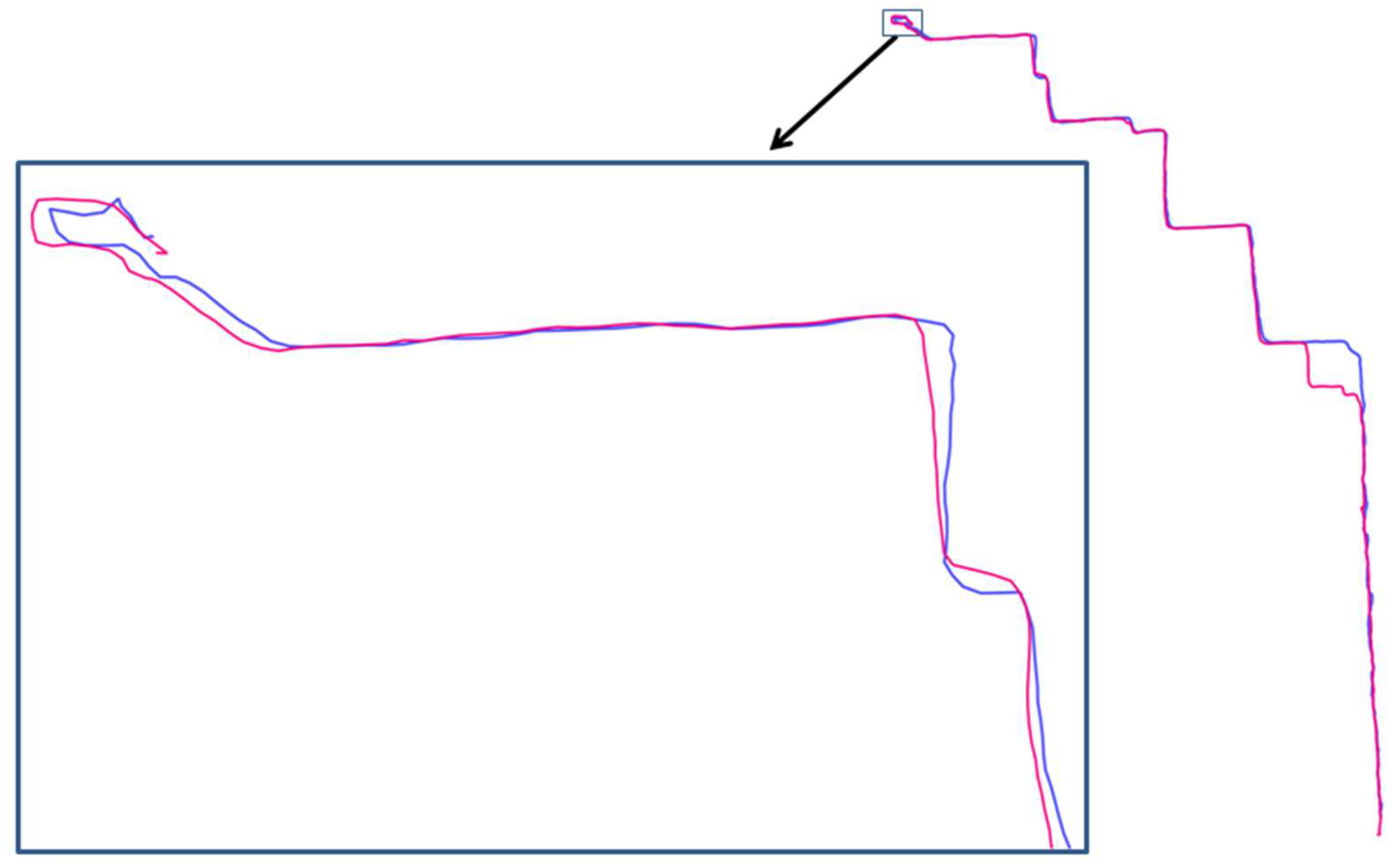
Self-intersection point: a self-intersecting point denotes a point where the trajectory passes through at least twice. A self-interacting point is considered to be a critical point as it encompasses some specific important properties: a self-intersecting point in a trajectory represents a node surely denoting the relative importance of that self-intersecting point. Among different parameters that can be considered for qualifying a self-intersecting point, the time and distance covered by the self-intersecting part of the trajectory between passing through twice can be mentioned.
Trajectory Critical Points are detected by the application of a Convex-Hull algorithm (TCP-CH) that has been applied to detect the main geometric characteristics, that is, curvature, turning and intersection points as introduced in our previous work [
58]. Prior to the application of the TCP-CH algorithm, noisy points are removed by the application of a Kalman filter whose objective is to smooth the successive positions by recursively correcting error values often generated by GPS positioning errors. Curvature and turning points are identified by the TCP-CH algorithm in such a way that starting and ending points of the convex hulls are selected as turning points, while for each convex hull the curvature point is the one located at the maximum distance from the connecting line of two turning points [
58].
Additional spatio-temporal properties are derived such as velocity changes and acceleration peculiar behaviors. Additional semantic descriptors are stop points as these are often connected to some worthwhile activities or bottlenecks. Stop-points are identified by the application of Dempster-Shafer theory and application of belief and non-belief functions [
59]. Besides the detection of these stop points, the uncertainty of the detection process is also considered. Overall, the velocity is derived for all relevant trajectory points. Therefore, without loss of generality, we introduce the following rule to identify a velocity change at a given trajectory point:
Rule 1.
There is a velocity change at the trajectory point ti of a trajectory T if and only if:where T(ti) and V(ti) respectively represent the position and velocity of a trajectory point ti, µi the velocity average for the trajectory points ti, ti−1, …, ti−10, β a parameter that denotes the expected magnitude of the velocity change (e.g., valued as 4/3 in the experiments developed). All the parameters listed above as well as the given times of the trajectory points denoted as Time
(ti) are detected and stored in a series of Abstract Trajectory Descriptor (ATD) representations that also consider the starting and ending points, as well as the critical points identified by the geometrical and semantic-based parameters.
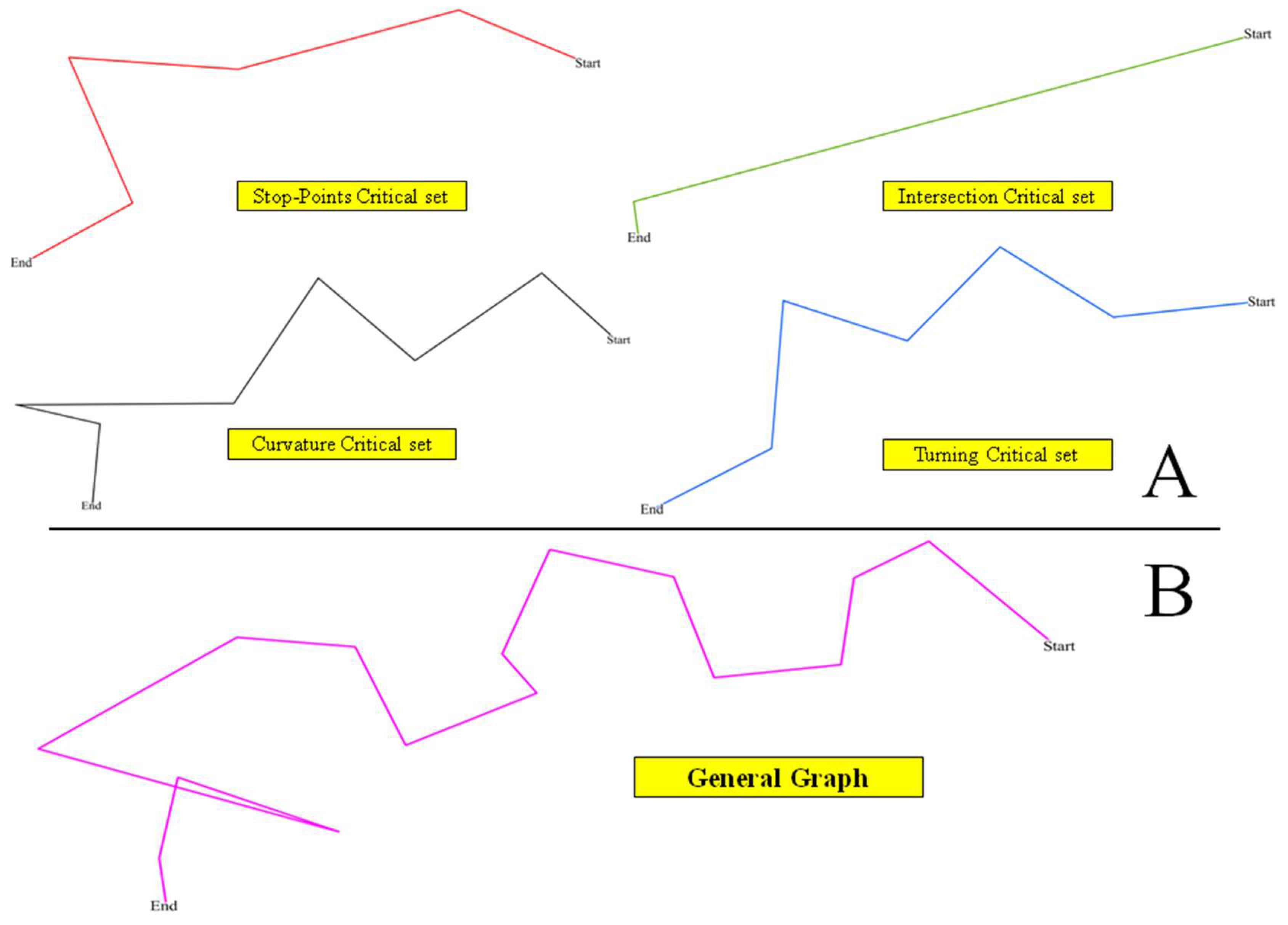
Figure 2A illustrates the principles behind the different trajectory critical points (i.e., self-intersections, direction changes, curvatures, stop points) and how such ATDs should be derived.
Figure 2B gives a schematic representation of the trajectory according to these critical points. The main principle behind this approach is to favor a comparison of several trajectories according to the parameters identified, and considering the underlying spatial and temporal properties embedded in these critical points.
3.2. Spatio-temporal Entropy Approach Principles
The STE-SD (Spatio-Temporal Entropy for Similarity Detection) approach developed is based on an application of the entropy theory which has been initially proposed for by Shannon as a probability distribution function to measure the data distribution in a given set of categorical data [
7]. The reasons behind this choice and application of the concept of entropy can be given according to the following motivations:
Not only the usual spatial distribution of the intermediate trajectory points should be considered, but also their temporal distribution. Next, additional parameters such as velocity should be considered in order to reflect some intrinsic changes in the trajectory.
Trajectories encompass some specific behavior reflected by critical points as identified by our approach (stop points, direction changes, curvature, self-intersections). Such critical points embed some spatial, temporal and semantic properties that represent some very specific behaviors that are crucial when cross-comparing several trajectories.
The reasons mentioned above leads us to search for and apply a measure of entropy that will reflect the spatial, temporal and semantic distribution of all these parameters within the intimate representation of some trajectories. The objective is to provide a sort of quantitative evaluation of such qualitative properties that will help to evaluate trajectory similarities and differences, and thus according to different configurationally parameters (as another objective is to provide a flexible evaluation approach).
While the measure of entropy as introduced by Shannon has been largely applied to the distribution of categorical data, it must be extended to the spatial and temporal dimensions to take into account the very peculiarities of space and time, and how the different parameters identified are related in space and time [
60]. In fact, we look forward a measure of entropy in space and time that can characterize the distribution and diversity of critical points embedded in a given trajectory. In a previous work, a related idea has been applied in Regional Science where a density-based analysis of the distribution of some entities has been developed [
61]. Nevertheless, what was required for this study is a comprehensive method that can overall consider the spatial and temporal distances among such critical points. To do so we applied a concept of spatio-temporal entropy introduced in a related work [
62]. The main idea of this notion of spatio-temporal entropy is derived from the first law of geography that states that “
Everything is related to everything else but near things are more related than distant things” [
63]. The different measures of spatio-temporal entropies suggested thus consider that the diversity of a given distribution in space and time will increase when different things are closed, whole the diversity will also increase when similar things are distant. The next section will develop the way the measures of spatio-temporal entropies can be applied to our critical-point-based representation of a trajectory.
3.3. Spatio-temporal Entropies
This goal of this section is to present how the concepts of spatial and temporal entropies can be applied to trajectory data according to the different measures of distances and critical points considered. As mentioned in the previous section, and as introduced in [
62] for a given configuration, the entropy value will increase when the distance between similar entities increases, or when the distance between different entities decreases. Accordingly, two concepts of internal and external distances have been suggested to derive such measure of spatial entropy [
62]. The
inner distance of a class
j denoted by
dj gives the average of the distances between the entities of this class
j. Similarly, the
external distance denoted by
dj represents the average of the distances between the entities of this class
j and the other entities that do not belong to this class
j. These respective inner distance (2) and external distances (3) are given as follows:
where
cj represents the set of entities of class
j, while
nj represents the cardinality of
cj.
N is the total number of entities,
di,j represents the distance between entities
i and
j.
To apply the principles of the
inner distance and
outer distance, let us consider the spatial distance
between two critical points
ti and
tj of a given trajectory
T. Hereafter, geometric and semantic descriptors introduced in the previous section are considered to be separate classes. Similarly, critical points are considered to be specific classes. This measure of spatial distance, as applied to the critical points of trajectory data, supports derivation of internal and external distances, and this for all classes of semantic and geometric descriptors. Let us therefore introduce the measure of spatial entropy as introduced in [
62], and as based on the measures of internal and external distances:
where
Hs is the measure of entropy,
pi is the percentage of entities in the class
i.
To apply this measure of spatial entropy we first evaluate the internal distance distribution of the critical points of a given class, and secondly the external distribution of the critical points of a given class with respect to the other critical points quantified by the measure of external distance. This will further provide a valuable direction to explore and quantify the possible similarities of different trajectories, and this according to some predefined critical points that encompass some specific semantic. For instance, curvature points reflect some specific properties of a given trajectory that can be cross-compared across several trajectories. Similarly, direction changes or self-intersections represent some specific behaviors when a human being is for example acting and moving in a given urban environment (or an animal behaving in a natural environment). Distances between such critical points often represent specific patterns. The frequency of the appearance of the different classes of critical points is another noteworthy trend to consider. These few examples show the variety of potential approaches for comparing the different semantic and spatio-temporal properties closely associated to some given trajectories. This is the reason for suggesting a flexible spatio-temporal measure of entropy that can outline such properties in different ways. The other option retained is to evaluate the ratio between the internal and external distances as given in Equation (4).
Similar to the way the measures of inner distance and outer distance have been applied to the spatial dimension, the measures of
internal temporal distance (5) and
outer temporal distance (6) have been also introduced to support the definition of a notion of temporal entropy [
62]:
where
and
respectively represent the internal and external temporal distances of the class
j, respectively, and where
. represents the temporal distance between two entities
i and
j as follows:
.
Next, the temporal entropy
for each trajectory
T is computed as follows [
62]:
where
pi denotes the ratio of the critical points of the class
i over all the classes.
The next goal is to introduce a spatial-temporal entropy matrix for all relevant trajectory data. The interest of this matrix is to give an overview of the different measures applied for a given set of trajectories. The dimensions of this matrix are ((2
m + 2) ×
n) where
n denotes the number of trajectories considered, and
m denoting the total number of semantic and geometrical parameters, and
T1,
T2,…,
Tn represent the id of trajectory 1, trajectory 2 and trajectory 2, respectively.
Table 3 presents the general structure of this matrix and the different critical points considered for each trajectory.
Finally, the measure of Spatio-Temporal entropy is computed as follows [
62].
with
And where
,
. and
denote the spatio-temporal entropy, spatio-temporal internal and external distances, respectively. Based on the entropy derivations introduced in
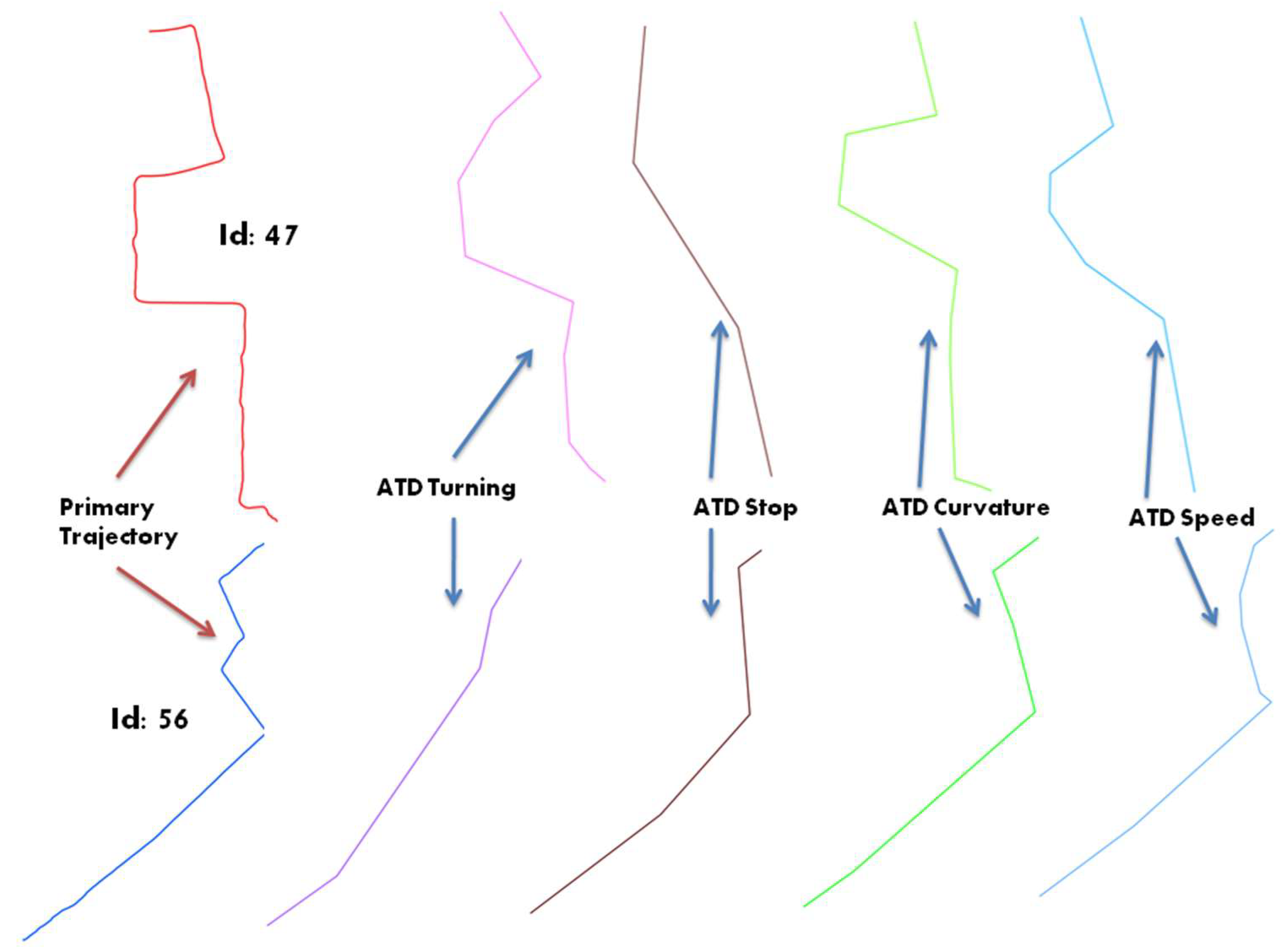
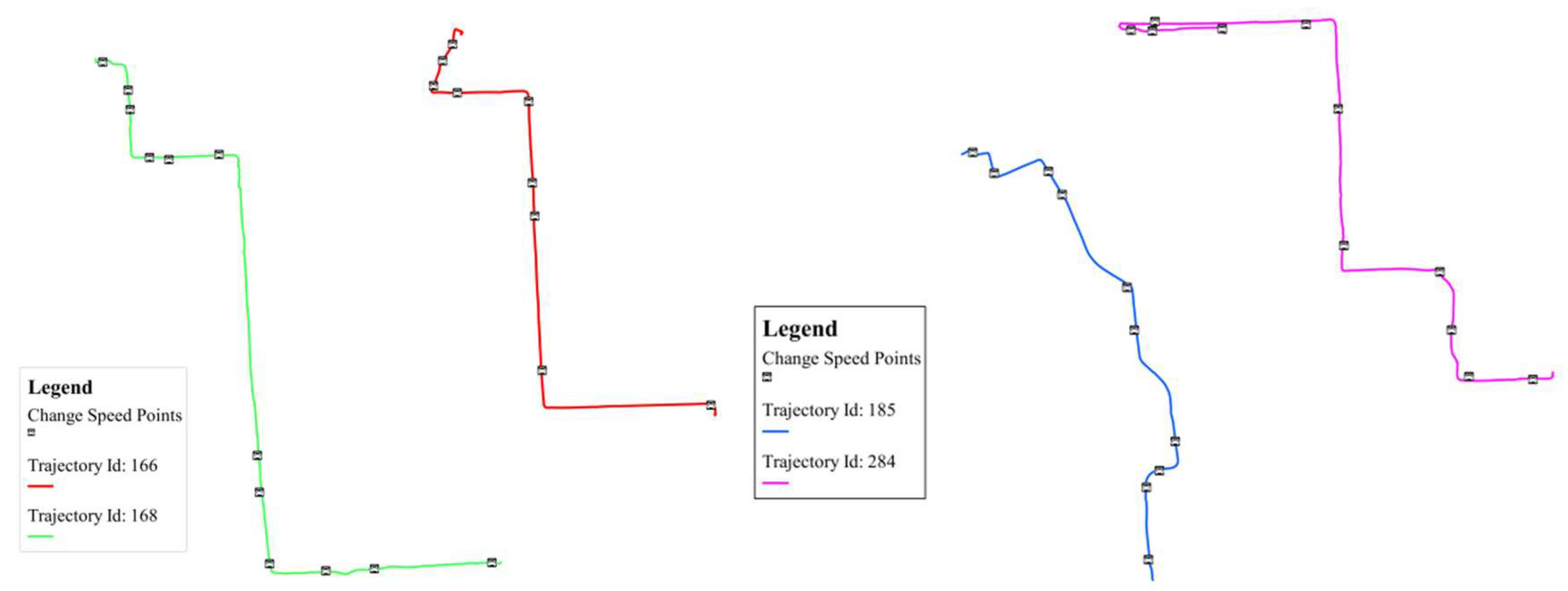
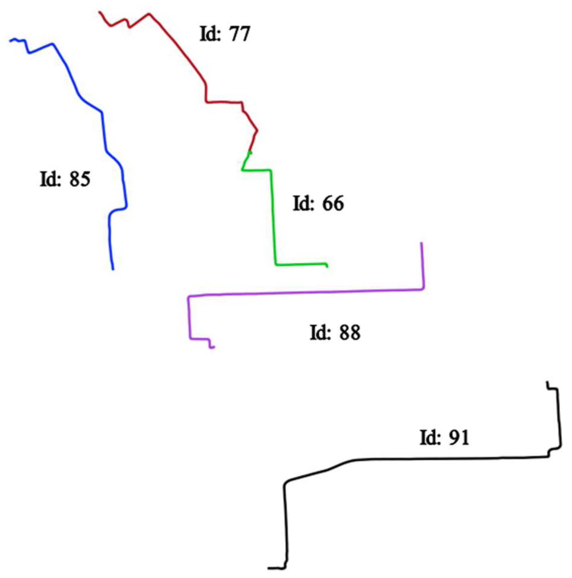
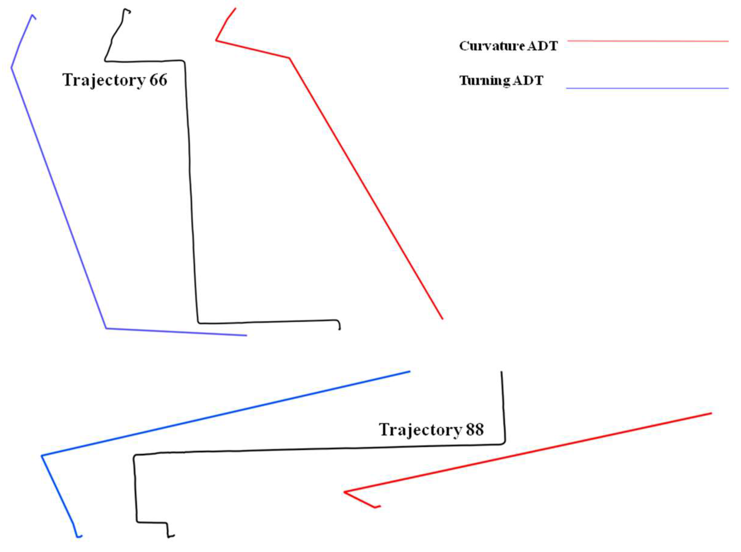
Table 3, each trajectory can be qualified using different spatial and temporal descriptors. Indeed, and depending on the application context, one might either consider some geometrical primitives such as curvature, turning or intersection points, or rather some spatio-temporal behavior such as trajectory speed changes. Let us for instance consider two trajectories extracted from the sample data and shown in
Figure 3. This schematic representation illustrates how these trajectories can be abstracted by considering different primitives, and then generating a sort of derived ADT trajectory representation.
As derived towards an ADT representation, each trajectory can be qualified by applying the measures of spatial and temporal entropies as presented in
Table 4.
The results presented in
Table 4 can be used to describe the semantics embedded in the trajectories 47 and 56, and for comparing them according to some preselected descriptors. For example, the results above outline a close similarity when considering the temporal dimension rather than when considering the spatial dimension.


