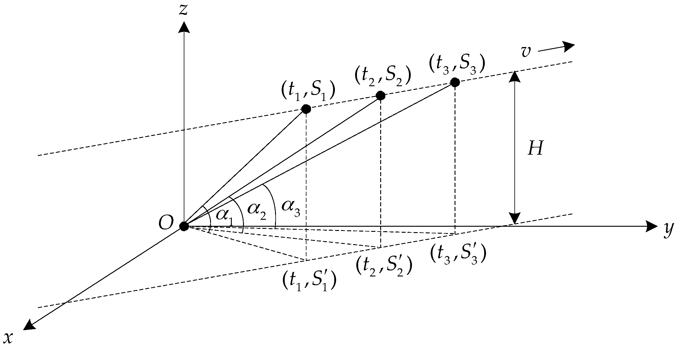
2.1. Doppler Phenomenon in the Stratified Media
A Doppler shift occurs when the source is in motion relative to the receiver. The Doppler frequency shift is related to the direction of the source movement, the signal frequency, the velocity of the source and the velocity of the medium. In
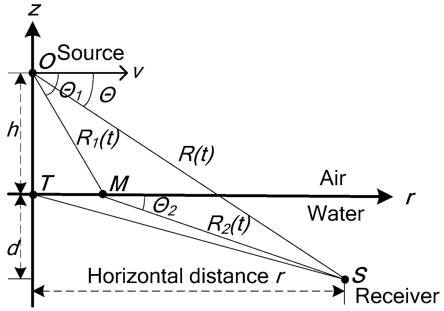
Figure 1, the source is located at the point
O, the underwater sensor (receiver) is located at the point
S, the point
M is the incident point of the direct refraction wave.
h is the height of the source relative to the sea surface.
d is the depth of the receiver relative to the sea surface.
T is the point just below the source in the sea surface.
R(
t) is the distance between the source position
O and the receiver position
S in the horizontal direction,
R1(
t) is the distance between the source position
O and the incident point
M in the horizontal direction,
R2(
t) is the distance between the incident point
M and the receiver position
S in the horizontal direction.
Assuming that the stratified medium is uniform and stationary, the source moves in the horizontal direction, and the Doppler frequency of the received signal is [
17]:
,
is the source frequency,
is the ratio of the source velocity
v to the medium velocity
c,
is the angle between the source-receiver direction and the source motion direction. Since
, then
,
, therefore
,
represents the received Doppler frequency,
represents the Doppler frequency offset,
.
In the horizontal stratified medium, according to the Snell theorem: , is the sound velocity in the air, is the sound velocity in the water. is the angle between the incident ray of the direct refraction wave and the source motion direction. is the angle between the refraction ray of the direct refraction wave and the source motion direction. The received Doppler frequency does not change. That is, the incident wave in the air and the refraction wave in the water have the same Doppler frequency.
When the source is located in the air and the receiver is located in the water, the sound waves received by the sensor consist of two parts: normal mode and non-uniform wave. The non-uniform wave transmits energy to the underwater receiver in a manner different from the refraction wave, as shown in
Figure 1. The normal mode arrives at the receiving point
S along the propagation path
OTS and the path
OTMS, while the non-uniform wave travels along the path
OMS to the receiving point.
Path
OMS: It is the transmission path of the normal mode in the air. This kind of wave is surface wave (non-uniform wave) below the air-water interface, its intensity decreases exponentially with the depth. This kind of wave is strong in the short-range. Its velocity signal has larger energy than its pressure signal, and has larger line spectrum Doppler shift. The Doppler frequency offset
is given by the following expression [
18]:
is the horizontal angle between the source motion direction and the sound propagation direction,
is the elevation angle.
Path
OTMS and
OTS: Path
OTMS is the transmission path of the normal mode whose eigenvalues are complex in the water and its Doppler frequency offset is
. The normal mode transmitting along the path
OTS in the water, is standing wave in the vertical direction of water,
is its Doppler frequency offset:
The instantaneous frequencies of the line spectrum signals arriving along the path
OMS and
OTMS are
and
, respectively [
18]:
The Doppler frequency offsets of the signals arrive along the OTMS and OTS paths are smaller, and their signal intensities are weak at the close range, so that during the frequency estimation process, the spectrum extraction of signals transmitting along the OTMS and OTS paths are more complex and more difficult, so in this paper, the line spectrum signal transmitting along the OMS path is the main research object.
2.2. Angle Estimation Method
The field contains pressure and velocity information, the former is the scalar field, while the latter is the vector field. Single point pressure is omnidirectional. For the traveling wave, the velocity signal matches the direction of arrival. The vector sensor is a kind of acoustic sensor used to measure the underwater vector field, which is made up of pressure sensor and velocity sensor (pressure gradient sensor, accelerometer, displacement meter, etc.) [
19]. The vector sensor outputs the pressure and the orthogonal three-dimensional (two-dimensional) velocity components [
20].
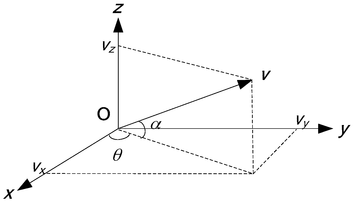
The three orthogonal components of the velocity
v are:
is the velocity waveform.
is the horizontal azimuth angle (range: 0–360°), the x-axis positive direction is 0°,
is the elevation angle (range: −90–90°), the horizontal plane (
xoy plane) is 0°.
Figure 2 illustrates the geometric relationship of the projection. If the pressure
meets
, the field is assumed to meet the Ohm law, then
.
is the target signal. According to (4), we can get:
In the discussion of signal processing problems, we can omit the acoustic impedance in the (5) and set .
The signal received by the underwater sensor is the refraction signal of the noise radiated by the aerial target. The expression of the received refraction signal is:
,
,
and
are the isotropic noise components of pressure and velocity received by the vector sensor, and they are all independent of
.
W is known as the refraction coefficient.
,
.
is the air density,
is the water density.
The physical basis of the complex acoustic intensity’s anti-interference performance is the correlation between the target pressure signal and the target velocity signal, whereas the pressure and velocity of isotropic environment interference is irrelevant or weakly correlated. The average output of the complex acoustic intensity is:
represents sliding-average periodgram operation. “
*” represents complex conjugate,
represents modulus operation, and
,
,
are the Fourier transform of the pressure and the velocity respectively,
is the Fourier transform of the signal,
is the Fourier transform of the interfere with the small quantity.
In the underwater acoustic channel, the acoustic Ohm law is approximately satisfied. Therefore, the pressure signal has the same phase as the velocity signal. According to the basic properties of the Fourier transform, the energy of the two signals in the same phase is concentrated on the real component of the cross spectrum. The imaginary component of the cross spectrum only contains the energy of interference and noise [
20,
21].
The cross spectrum method at single frequency point is given by:
represents the operation of getting the real component.
In this paper, we use the weighted bar graph method to do the statistical analysis of the azimuth estimation results. The specific algorithm of the weighted bar graph method is given by:
is the azimuth sequence in the angle domain,
represents the getting integer operation towards positive infinity,
represents the modulus operation,
is the azimuth estimation value at every frequency point,
k is the sequence number of the frequency point,
M is the total number of frequency points used in the azimuth estimation.
is the complex acoustic intensity of the
k-th frequency point.
Z is an array whose dimension is 1 × 360. We use the array
Z to do the weighted statistic of the azimuth sequence
. The complex acoustic intensity
, used for summation in (12), meets
.
n is an angle sequence which varies from 1° to 360°.
Using the azimuth estimation method based on (9), we can calculate the azimuth value at every frequency point. Then we use the weighted bar graph method to do a statistical analysis of the azimuth estimation result at every frequency point, so as to get the probability distribution of the azimuth estimation at a certain time. The azimuth corresponding to the maximum value of the probability distribution is the desired target azimuth.
In this section, we introduce the angle estimation method with a single vector sensor in the horizontal direction, namely, we give the estimation method of the azimuth angle. The angle estimation method in the vertical direction (elevation angle) is introduced in the
Section 3.1.
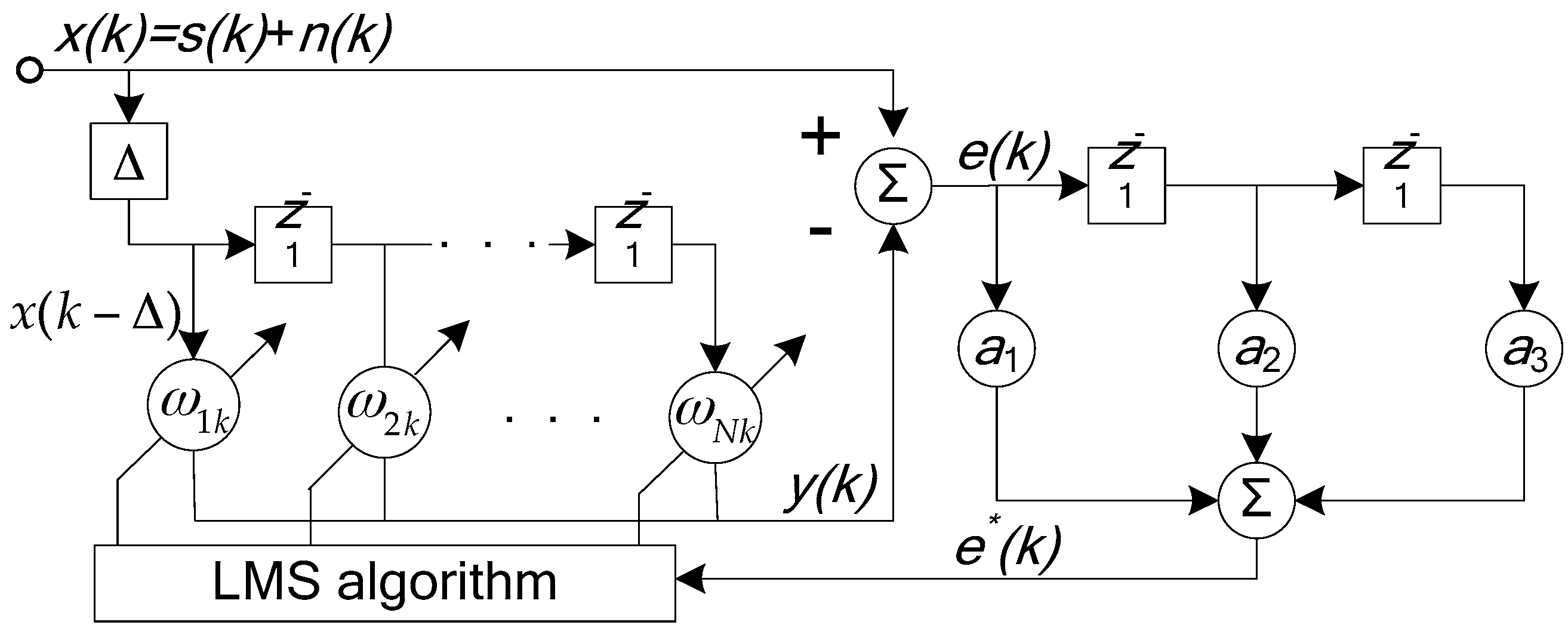
2.3. Frequency Estimation Method
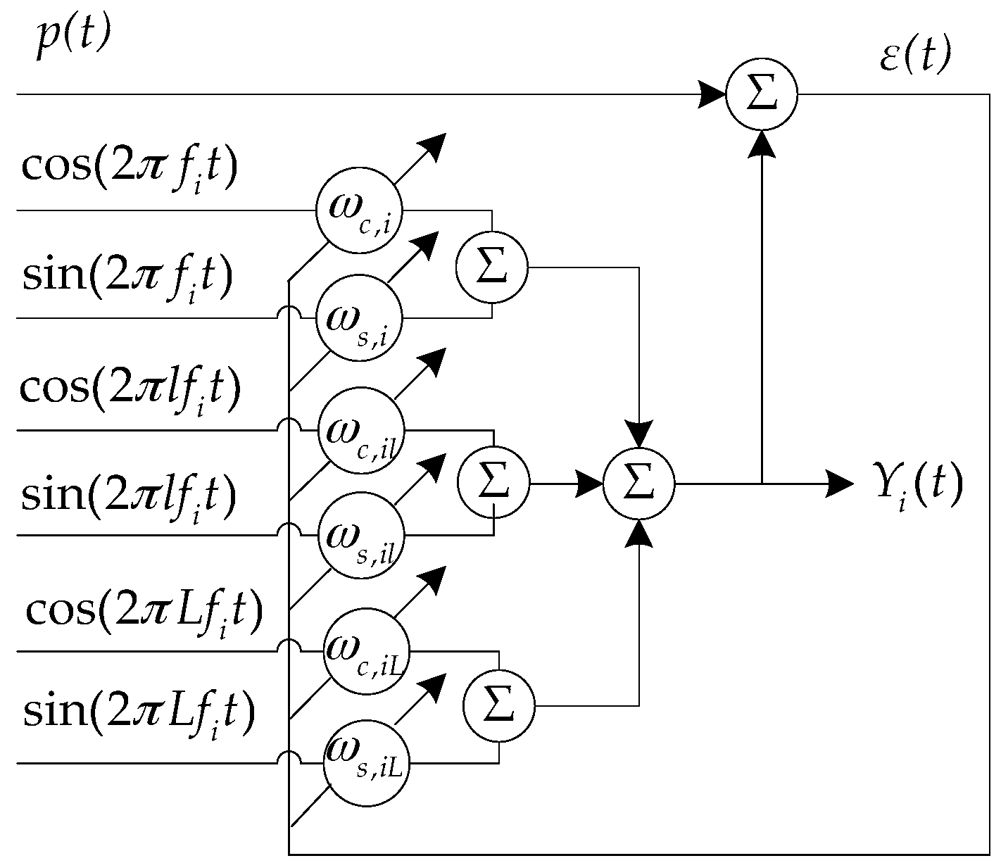
In this paper, we use the harmonic cluster adaptive line spectrum enhancer to extract the aerial target base frequency [
22]. Assuming that the aerial target signal consists of harmonic cluster line spectrum whose shaft frequency is
, the modulation line spectrum cluster is:
is the shaft frequency, there are
N harmonic components;
n takes from the natural number between 1 and
N;
t represents the time;
n(
t) represents the background noise signal.
Figure 3 shows the structure of the harmonic cluster adaptive line spectrum enhancer. By frequency sweeping, the harmonic component of the input signal can be enhanced when the harmonic component of the input signal
p(
t) corresponds to the frequency of the harmonic cluster reference input signal. The input signal is
p(
t), the shaft frequency of reference signal is
, the scanning step is
. We start scanning from the low frequency. Each scanned harmonic cluster has
L sets of reference input signals. Two reference signals of the each set of input signals are mutually orthogonal. Respectively, they are:
the center frequency of each set of reference signals is harmonically related.
l takes the natural number between 1 and
L. Adjust the base frequency
of the harmonic cluster. The range of
is the frequency range of the shaft frequency. During each scanning of the base frequency, the harmonic cluster is accumulated, the iterative formula of the weight vector is:
is the harmonic cluster adaptive line enhancer (ALE) output at the base frequency;
and
are the
L × 1 order weight vectors whose initial values are both 0.
.
is a constant parameter whose value is 0.001. When the base frequency
of the harmonic cluster or its harmonic frequencies do not coincide with the line spectrum, the frequency spectrums at the frequency of
and its harmonic frequencies are not enhanced, the noise is not enhanced too. After the sweep processing in the whole frequency band, when
, the system output line spectrum energy is the largest, through the spectrum level signal noise ratio (
SNR) maximum criterion, the harmonic cluster adaptive line spectrum enhancer’s best output can be selected. At this time, the reference base frequency
is the shaft frequency of the target.
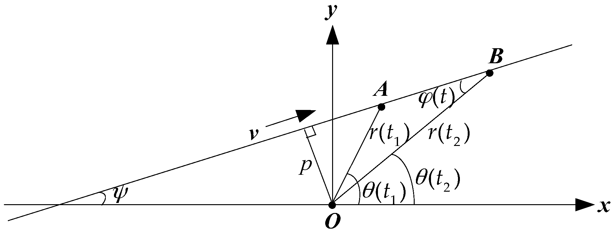
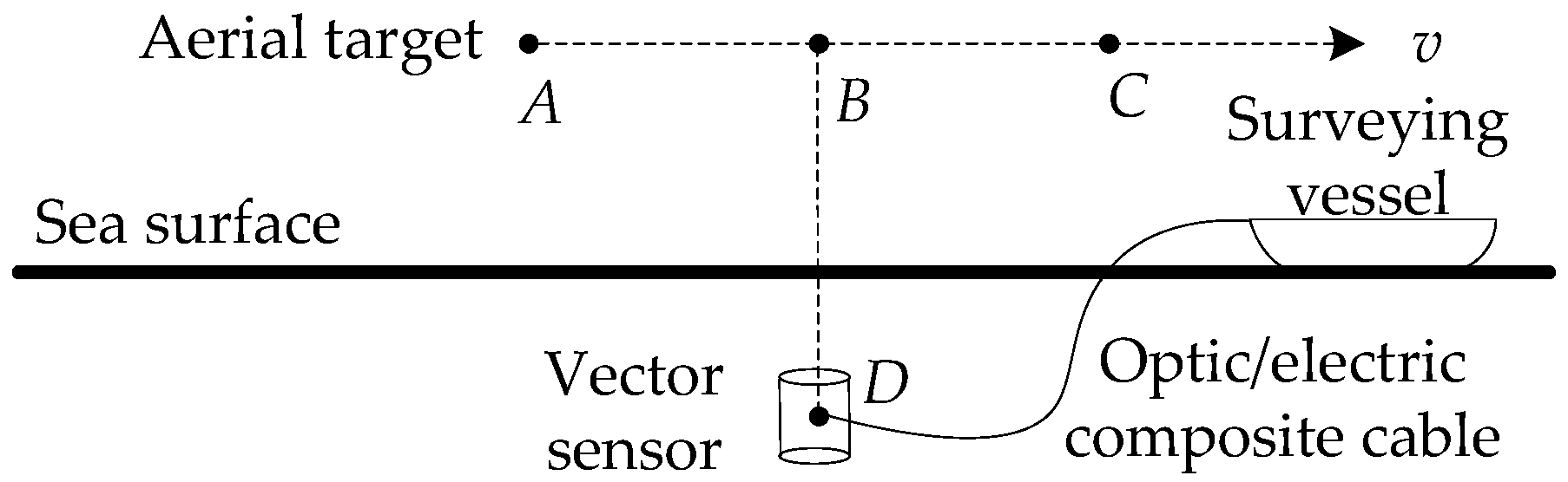
2.4. Geometric Relationship of Passive Localization in the Horizontal Direction
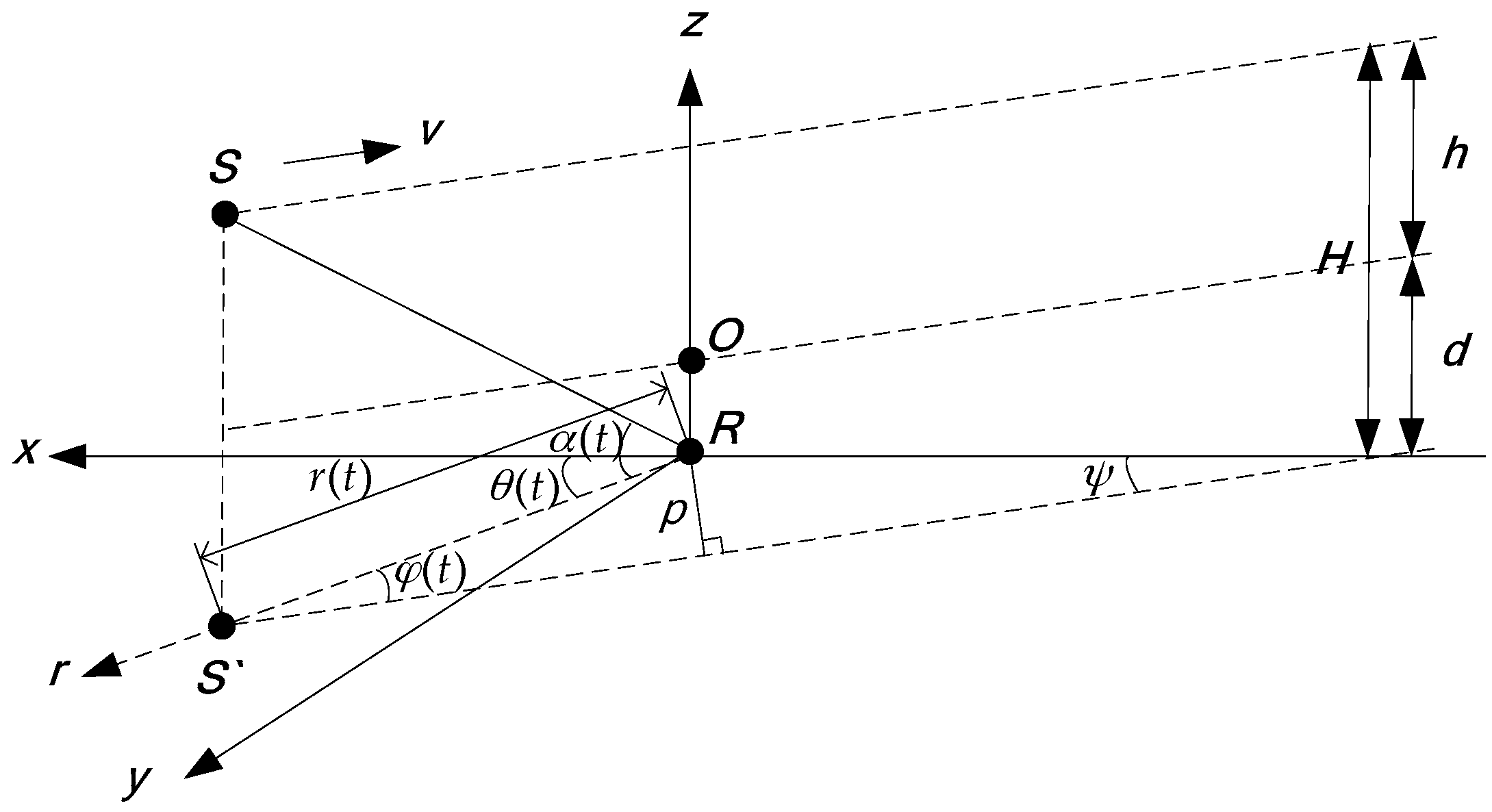
Assuming that the aerial target, located at the point
S, is flying at a constant altitude
h (the reference surface being the sea surface), and moving on a straight line at the constant velocity
. The depth of the underwater sensor, located at the point
R, is
(the reference surface: the sea surface). The projection of
S at the
xoy surface is
. The point
R is considered as the origin of the Cartesian coordinate system.
O is the point directly above the receiving sensor in the sea surface.
H is the vertical distance between the source and the receiving sensor. The passive localization geometry relationship is shown in
Figure 4. In this paper, all of the following horizontal distances are the distances between the source and the receiving sensor in the horizontal direction, and all of the following vertical distances are the distances between the source and the receiving sensor in the vertical direction.
is the target horizontal distance,
p is the closest horizontal distance,
is the angle between the motion path and the x-axis positive direction, and
is the target horizontal azimuth angle.
is the angle between the source motion direction and the sound propagation direction.
is the target elevation angle in the vertical direction. Taking any reference time
t = 0, the position at this time is
, the target azimuth is
. The horizontal distance is
.
The motion equations in the
xoy plane are:
,
and
are the two orthogonal components of the velocity
,
,
,
,
,
,
,
. In polar coordinates, the straight line equation is
. Therefore, it can be seen from the above formulas that the passive localization can be realized after obtaining the values of
in the actual measurement [
23].
In the geometrical schematic diagram of passive localization shown in
Figure 4, the position of the receiver is the origin of the coordinate, and in the direct refraction wave ray trace shown in
Figure 1, its coordinate origin is the incident point of the refraction wave. When the direct refraction wave is used as the main research signal of the passive localization, the direct refraction wave ray trace (
OMS) is approximated to the line from the source to the receiver in this paper. The ray trace of the direct refraction wave shown in
Figure 1 can be simplified to the ray trace in the passive geometrical schematic diagram shown in
Figure 4. It can be seen from the geometrical relationship of
Figure 1 and
Figure 4 that, in the horizontal direction, the horizontal component of
is
, that is, the approximation does not change the magnitude of the horizontal distance and does not affect the estimation accuracy of the horizontal distance. It can also be seen that, in the vertical direction, the vertical component of
is
, namely, the approximation does not change the magnitude of the vertical distance and does not affect the estimation accuracy of the vertical distance. The relationship between
and
,
is
.
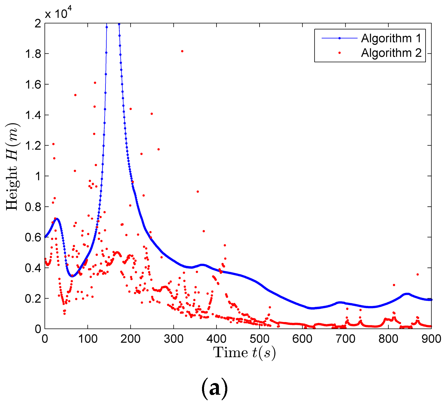
2.6. The Basic Principle of the Improved Parameter Estimation Algorithm
The simulation results of the algorithm shown in
Section 2.5 are very good, but in the practical application, the algorithm cannot achieve the effect in the simulation because of the limited azimuth and elevation estimation accuracy, so the following improvements are made to the algorithm.
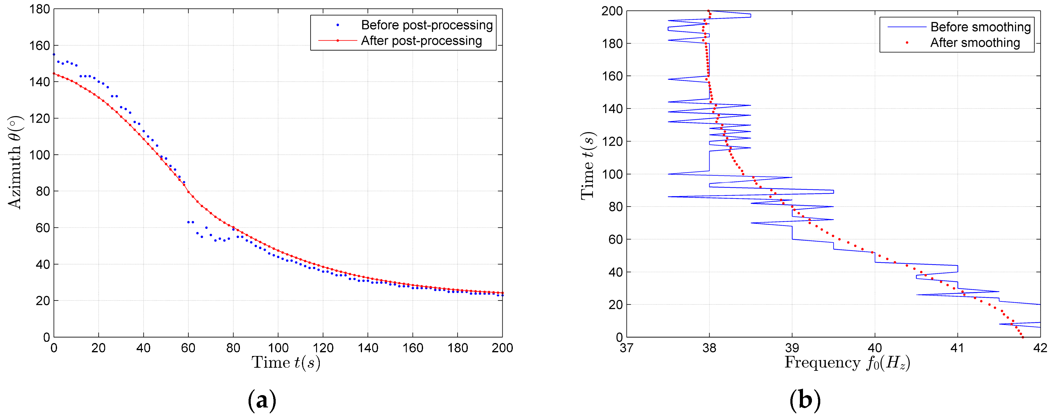
2.6.1. Improvement of the Frequency Estimation Algorithm
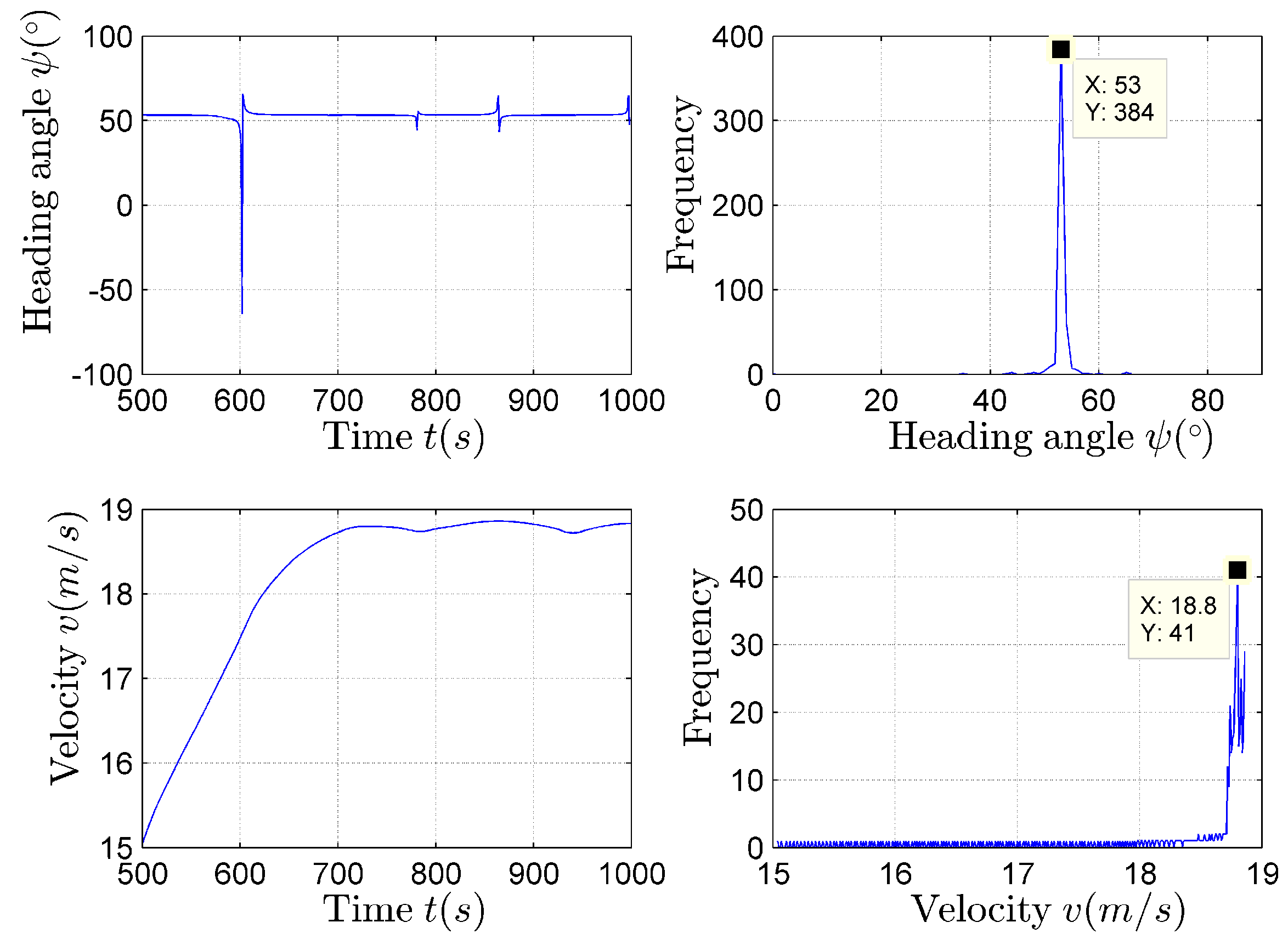
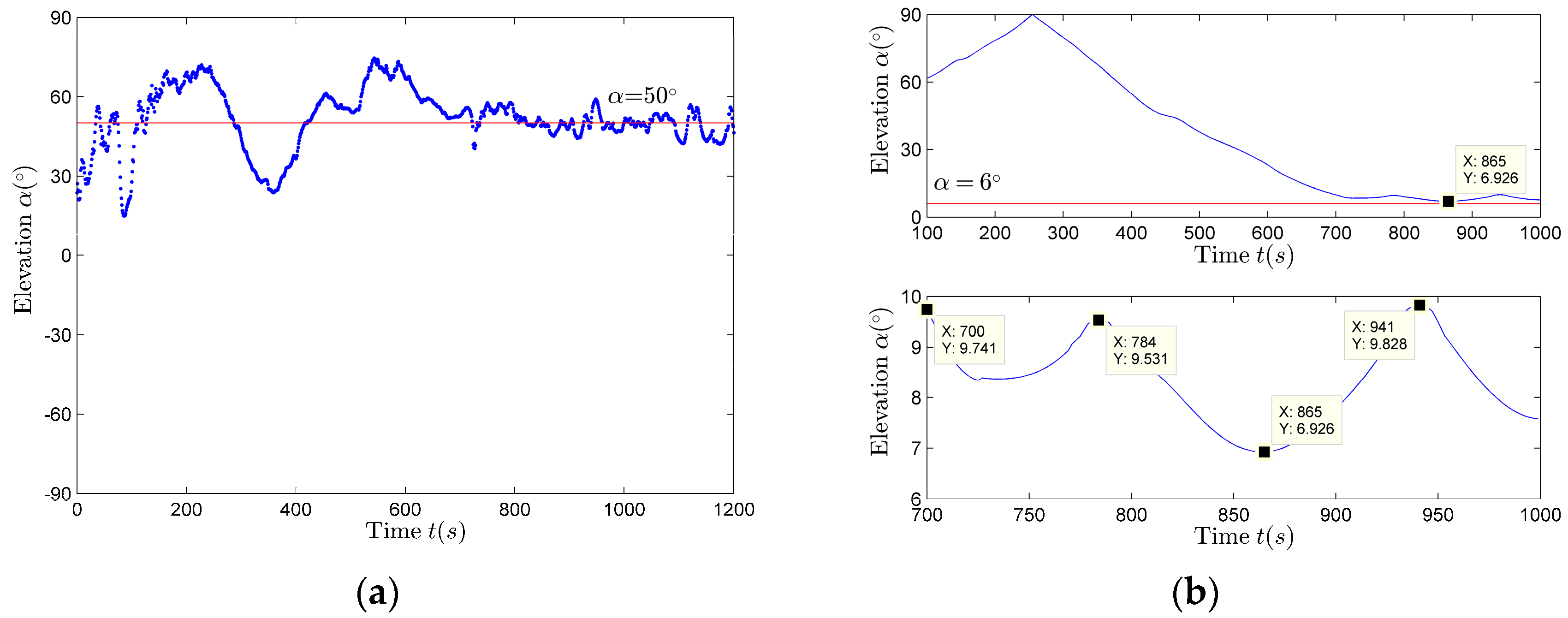
If the frequency estimation is made using (18), the estimation effect is poor when the azimuth changes slowly, namely
, and many maxima are estimated because there is a phenomenon that the denominator is approximately zero. The algorithm is improved by using the least squares method to fit the extracted spectrum sequence
, so as to obtain the fitting result
. Select the appropriate time period to estimate the base frequency. Firstly, the selected time period should satisfy that the frequency, which is almost constant, cannot account for a large proportion, otherwise the estimation result is that stable value. However, the stable value is generated when
, at this time
, the base frequency estimation result
is not the source frequency
which is of great need. According to the time distribution curve, apart from meeting the above conditions, the selected time period for the base frequency estimation should be away from 0 and stable:
Compared with using for subsequent parameter estimation, using for subsequent parameter estimation has a better estimation effect.
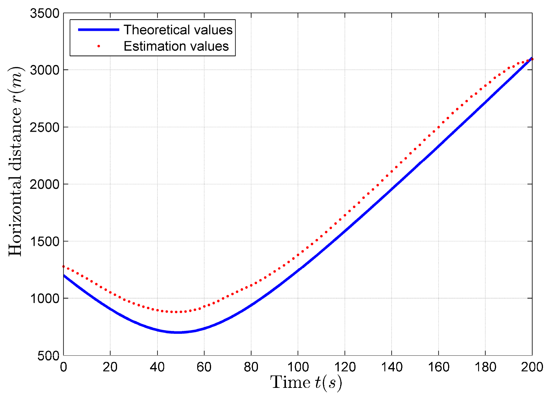
2.6.2. Improvement of Closest Distance Estimation Algorithm
In the estimation process of the closest horizontal distance p, there is also a problem that the estimation effect is poor when the azimuth changes slowly, because , then , so the denominator of (21) is approximately zero, and there are a large number of maxima in the estimation results.
In this case, the estimation results obtained by using (21) cannot achieve the expected accuracy, so the algorithm should be modified as follows: in the time period when the horizontal distance is close to the closest distance, the following approximation is used:
Since
,
, thus in the triangle
OAB shown in the
Figure 5,
,
.
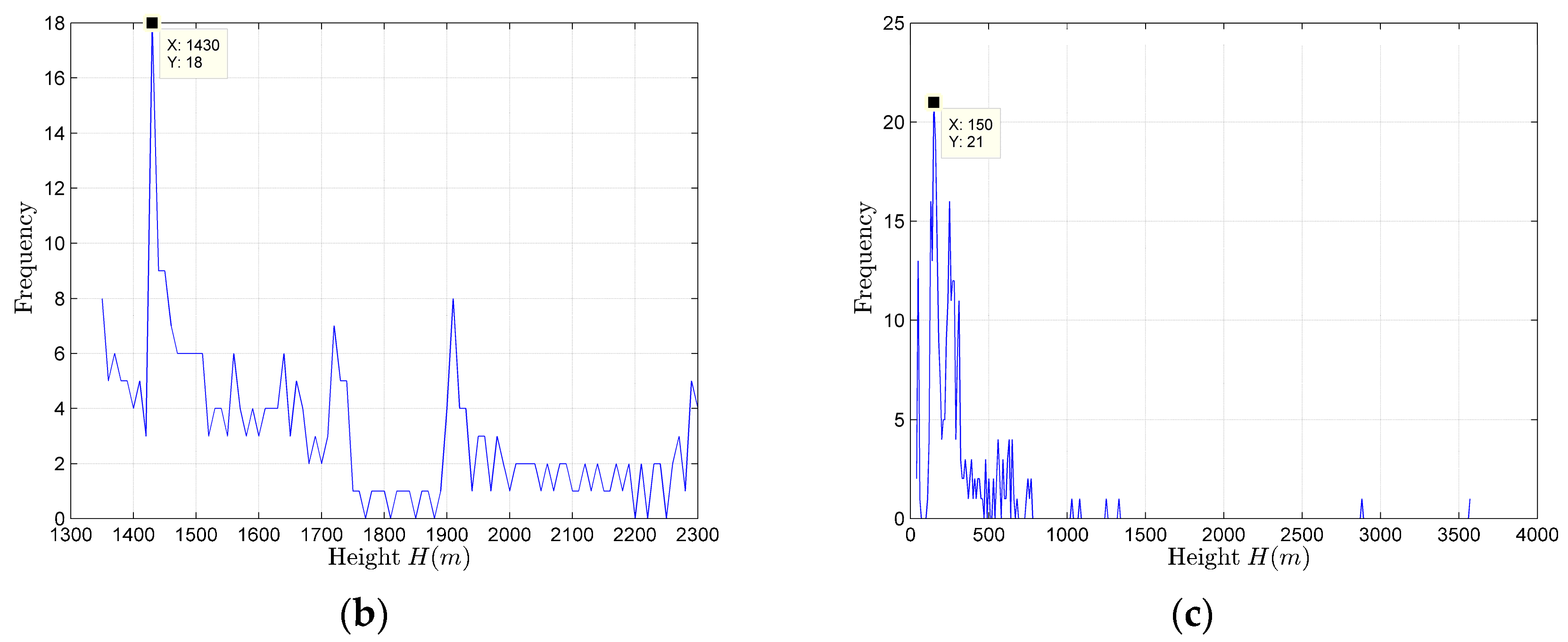
In this case, we use the matching algorithm to calculate the requested p value. The concrete steps of the matching algorithm are the following:
Assume a value and obtain the corresponding estimation curve according to (22). Because the magnitude of the value only affects the amplitude of , value does not affect the variation trend of .
According to the curve, the more stable time period can be determined.
Through matching estimation at the selected interval, scanning each value, the corresponding velocity estimation sequence can be obtained.
The mean value of the velocity estimation results in the stable time period is taken as the estimated value corresponding to the scanned value.
When the value is closest to the velocity estimation result obtained through using (20), the corresponding is regarded as the optimal estimation result of the closest distance.
After obtaining the optimal estimation result of , according to (22), the estimation is still found to be discontinuous, and there are still quite a lot of maxima. Since the estimation is inaccurate and discontinuous, using the data at the previously determined stable time period as the initial data, after compensating the subsequent data, we can obtain more continuous and better estimation results.
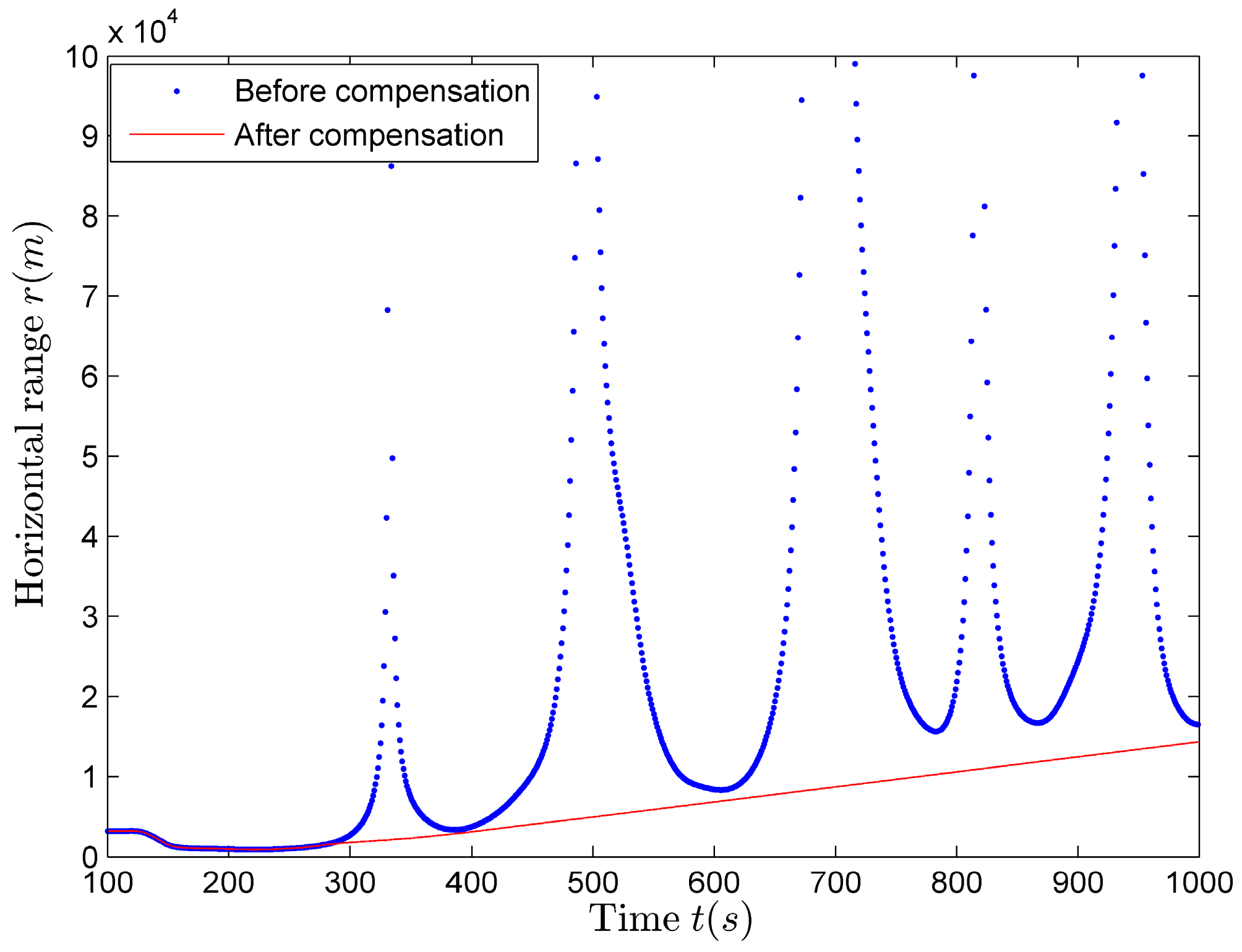
2.6.3. Horizontal Distance Compensation Algorithm
in the steady time period is used to compensate the subsequent estimation results. The appropriate time point
, in the steady time period, is used as the starting time. The compensation result of
is calculated as follows:
Using the above parameter estimation formulas, as long as we estimate the azimuth sequence and frequency sequence, we can carry out the corresponding parameter estimation.


