In this section, the proposed method is first illustrated. Then, the related theories such as the RBM and the ELM are presented in detail.
2.1. The Proposed Method
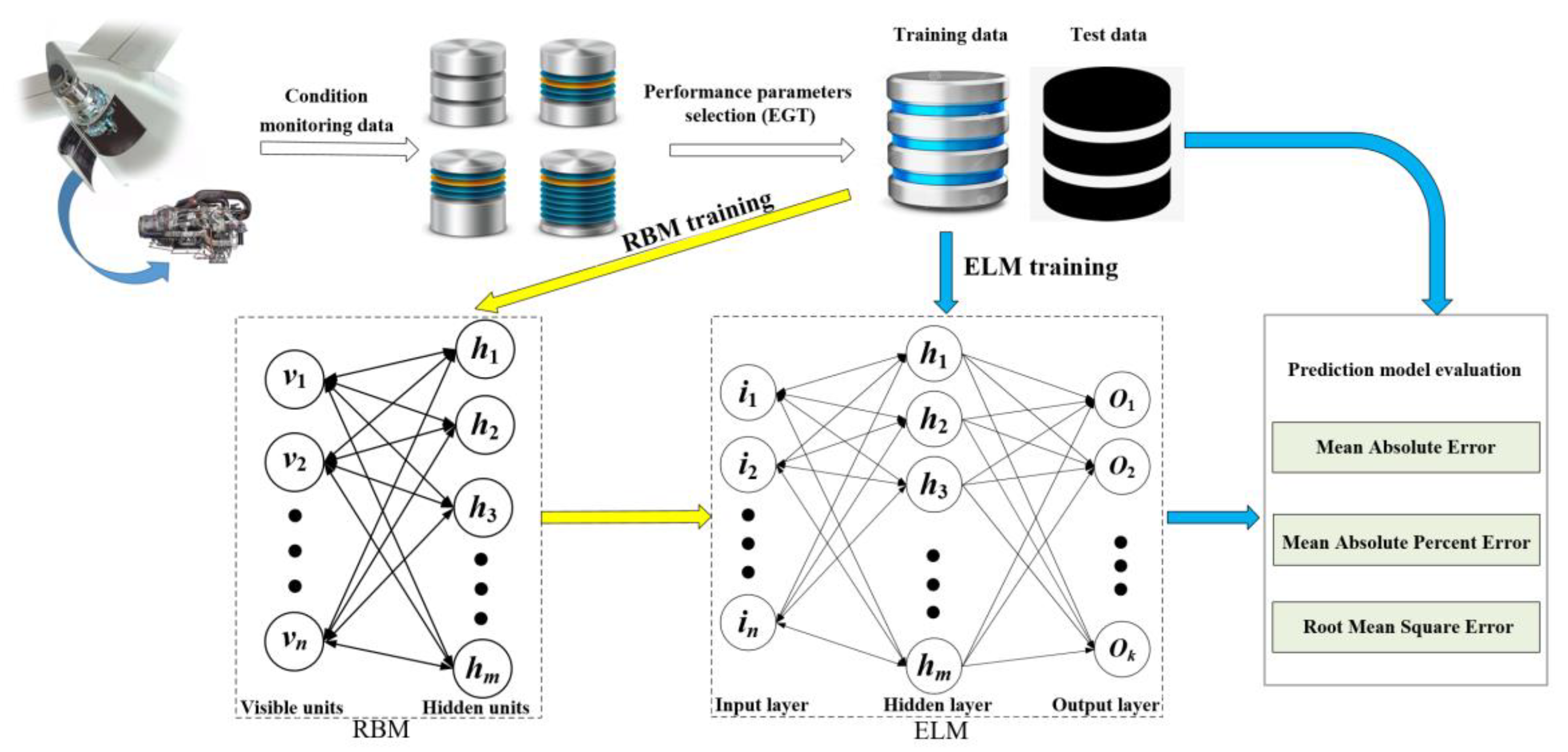
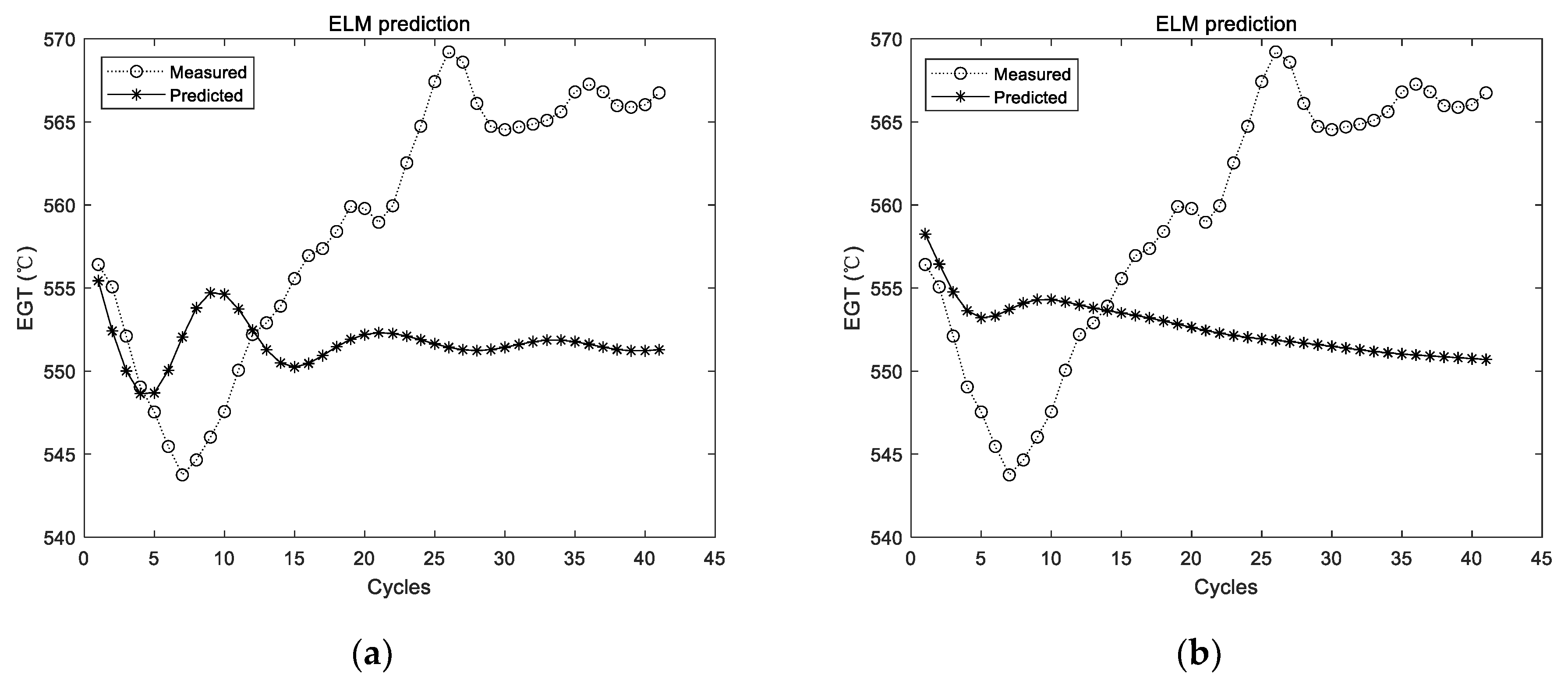
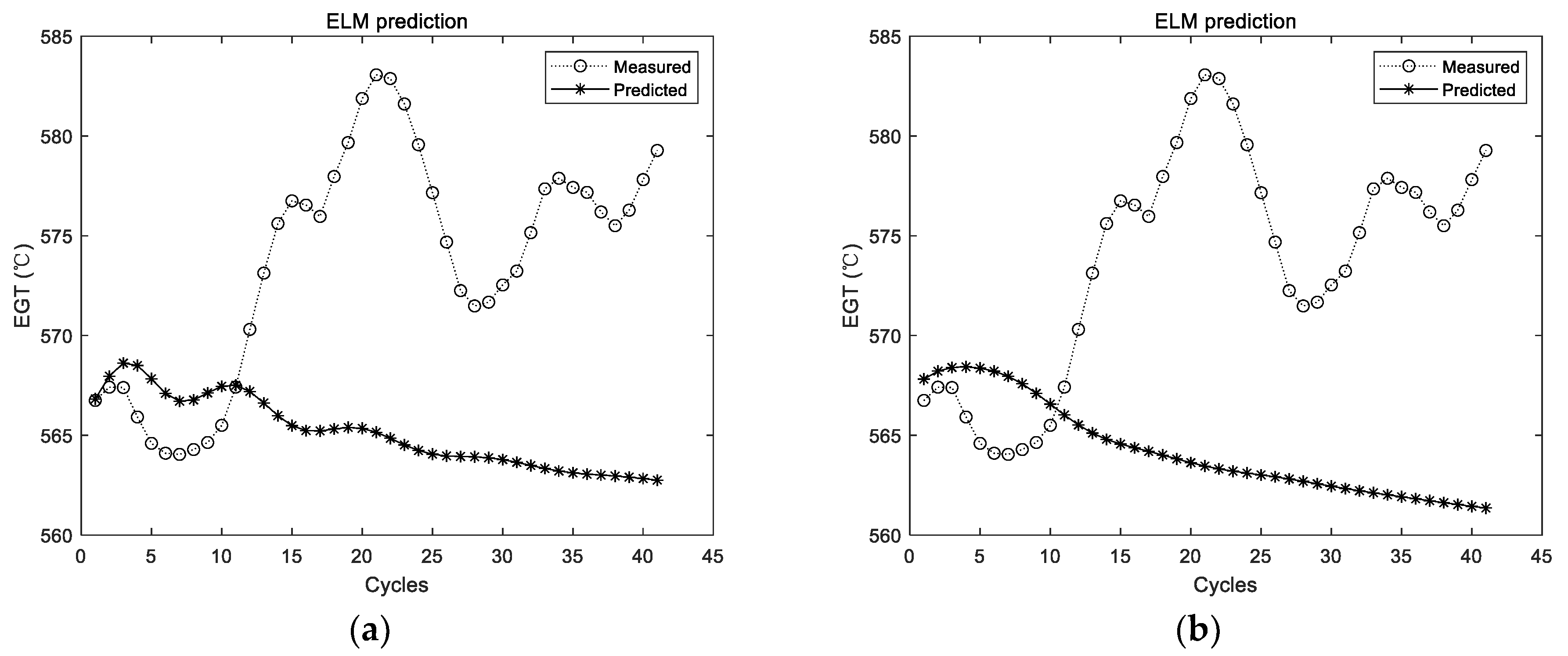
The ELM has the advantages of a faster learning speed and better generalization performance. To deal the problem of slow training of neural networks with the back propagation algorithm, an ELM was adopted to predict the performance sensing data of the APU in this study. However, the randomly generated weights and thresholds of the ELM often lead to unstable prediction results. To address this problem, an RBM was utilized to optimize the connection weights and the thresholds between the input layer and the hidden layer. In this way, a stable performance sensing data prediction model of the APU is expected to be achieved. The prediction results can also be obtained, and better prediction can be realized. The proposed method is illustrated in
Figure 1.
To conduct the proposed method, the specific procedures are explained as follows.
Step 1. Choose the EGT data as the key parameter of the performance sensing data, which are from condition monitoring data of the APU. Preprocess the original data and divide the preprocessed data into training data and test data, respectively.
Step 2. Initiate the related parameters of the RBM and train the RBM with the available data.
Step 3. After the RBM is well trained, the weights and thresholds of the RBM are assigned to the ELM.
Step 4. Utilize the training data to train the ELM. In this way, all parameters of the ELM can be determined.
Step 5. Predict the EGT of the next cycle based on the historical EGT. The predicted EGT data are used as part of the historical EGT. These combined data are utilized to predict the EGT of the next cycle. This process is repeated until the preset prediction steps are met.
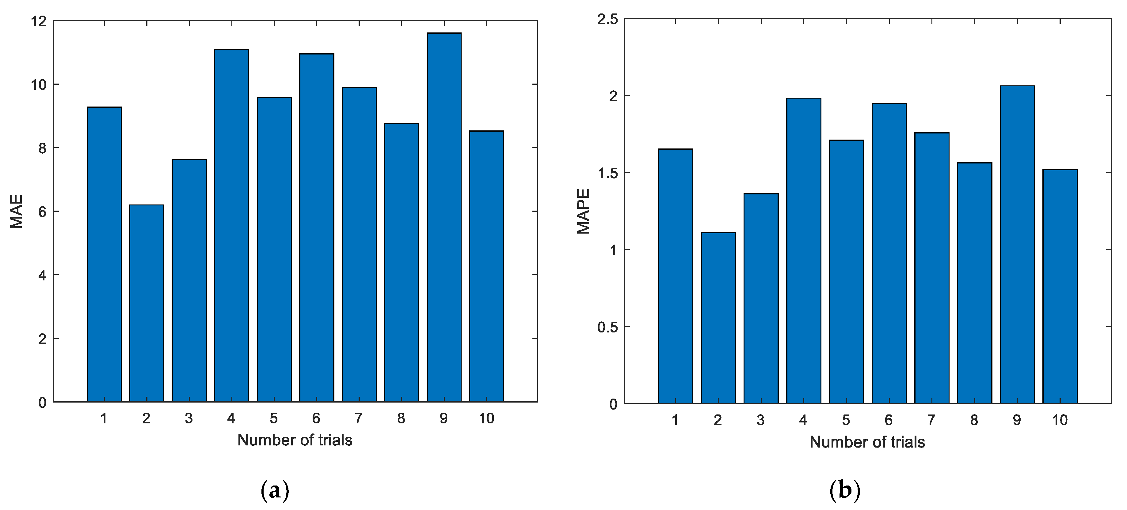
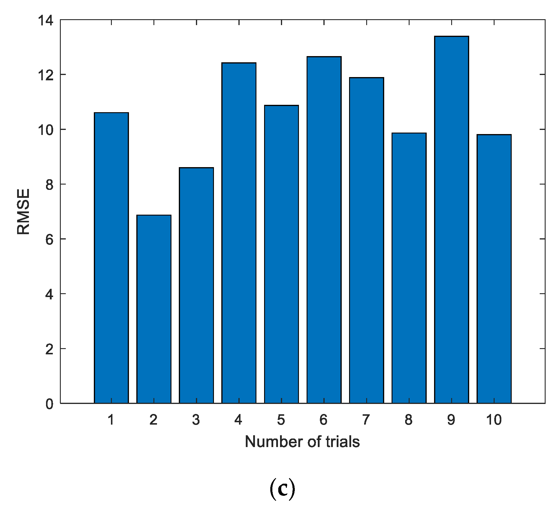
Step 6. Evaluate the prediction results by appropriate metrics.
The error function in the ELM can be regarded as an energy function. In general, the optimal solution of network parameters can be obtained using the generalized inverse algorithm. However, if the weights and thresholds of the input layer and the hidden layer are generated randomly, the ELM network often falls into the local minimum point but fails to reach the global minimum point. The reason is that the error function or energy function of the network is a nonlinear space with multiple minimum points, and the random weight and threshold generated by the ELM will cause the network to fall into the local minimum value due to its randomness. Compared with the ELM, the main difference between a random network (e.g., RBM) and the ELM lies in the learning stage. Unlike other networks, a random network does not adjust weights based on a certain deterministic algorithm but modifies according to a certain probability distribution. In this way, the aforementioned defects can be effectively overcome. The net input of a neuron does not determine whether it is in a state of 1 or 0, but it does determine the probability that it is in a state of 1 or 0. This is the basic concept of a random neural network algorithm.
For the RBM network, with the evolution of the network state, the energy of the network always changes in the direction of decreasing in the sense of probability. This means that although the overall trend of the network energy is to evolve in the direction of a decrease, it cannot be excluded that some neuron states may have a value with a small probability. Thus, the network energy is increased temporarily. It is precise because of this possibility that the RBM network has the ability to jump out from the local minimum trough, which is the fundamental difference between the RBM and the ELM. This operation is called the search mechanism, which means that the network is in the process of running a continuous search for lower energy minima until the global minimum of the energy is achieved.
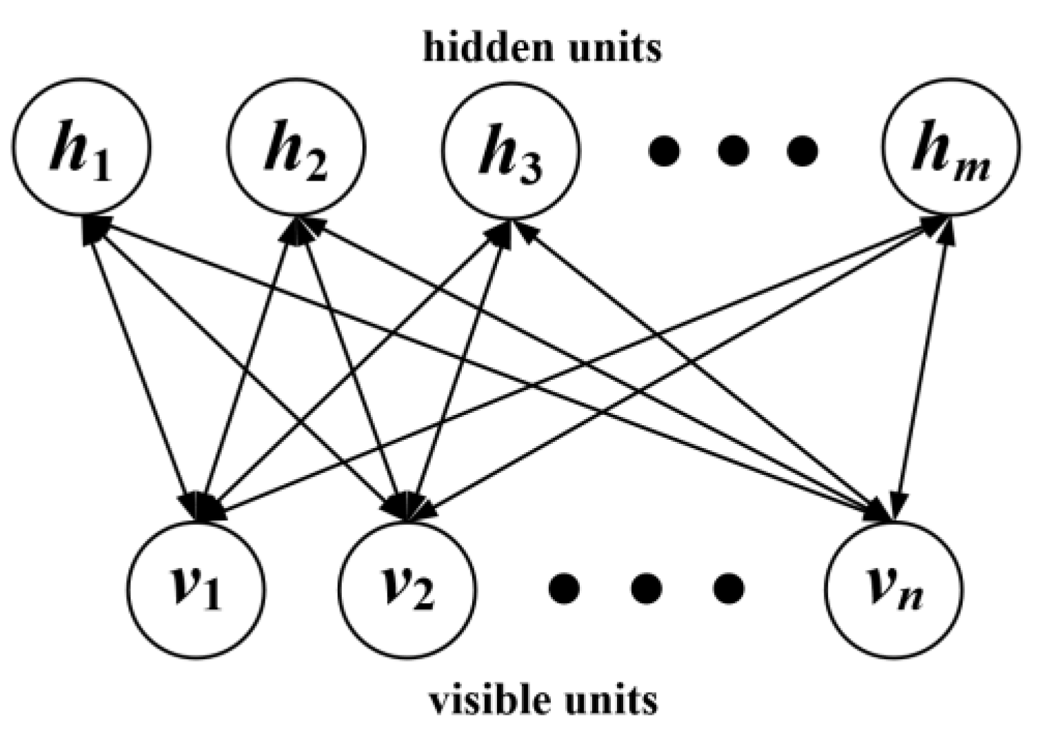
2.2. Restricted Boltzmann Machine
The RBM has only two layers of neurons, as shown in
Figure 2.
The first layer is named as the visible layer, which consists of visible units for training data input. The other layer is named as the hidden layer, which consists of hidden units.
If the RBM includes
n visible units and
m hidden units, the vectors
v and
h can be used to represent the states of the visible and hidden units, respectively.
denotes the state of the unit
i in the visible layer and
is the state of the unit
j in the hidden layer. For the set
, the energy of the RBM is defined by
where
is the parameter of the RBM, and
represents the connection weight between visible unit
and hidden unit
.
is the bias of the visible unit
, and
represents the bias of the hidden unit
. When the parameters are determined, the joint probability distribution of
can be obtained by
where
is the normalized factor (also known as the partition function). The distribution
of observed data
v defined by the RBM is the essential issue. To determine this distribution, the normalized factor
needs to be calculated.
When the state of visible units in the RBM are given, the activation state of each hidden unit is conditionally independent. At this point, the activation probability of the unit
j in the hidden layer is
where
is the sigmoid activation function. Since the structure of the RBM is symmetric, the activation state of each visible unit is also conditionally independent when the state of the hidden units is given. The activation probability of the unit
i in the visible layer is
It should be noted that there are no interconnections among the neurons in the visible and hidden layers. Only the inter-layer neurons have symmetrical lines and their relationship is independent, as given by
When the hidden layer is given, all explicit values are not related to each other, as illustrated by
With this property, it is not needed to calculate each neuron at every step. Instead, the neurons in the entire layer can be calculated by the parallel mode.
The training target of the RBM is to find the maximal probability distribution of hidden units with the training sample. Since the decisive factor lies in the weight W, the object of training the RBM is to determine the optimal weight.
The marginal distribution of joint probability distribution
P is the likelihood function, as defined by
When the training data
D are given, the goal of training the RBM is to maximize the following likelihood:
Equation (9) can be equivalent to
A random gradient descent can be applied to solve the former problem. The derivative of
with respect to
needs to obtained, as illustrated by
The first term corresponds to the expectation of the energy gradient function under the conditional distribution . The second term corresponds to the expectation of the energy gradient function under the joint distribution .
The first term is easily calculated. However, represents the joint distribution of visible layer units and hidden layer units, which involves the normalized factor Z. This distribution is difficult to obtain. Therefore, we cannot calculate the second term, only its approximation can be achieved through some sampling methods.
Then, Equation (12) can be obtained, as given by
When
equals
, we can get
When
equals
, the following equation can be reached:
When equals , Equation (15) can be achieved.
Finally, the following three equations (Equations (16)–(18)) can be derived.
The computational complexity of
in the above three equations is
. Therefore, the Markov chain Monte Carlo (MCMC) method, such as the Gibbs sampling method, is usually adopted for sampling, and uses samples to estimate
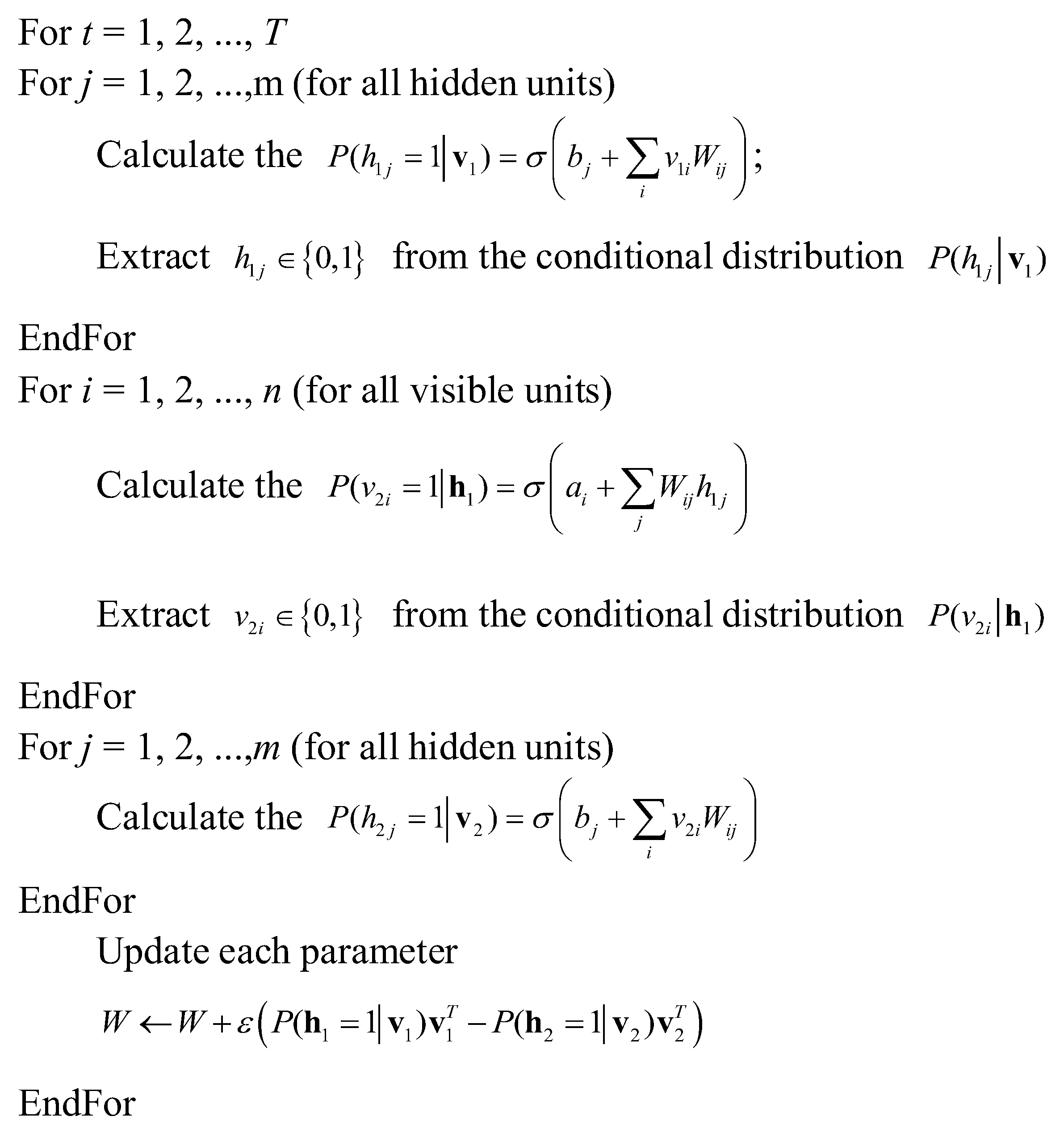
. However, each time MCMC sampling is performed, sufficient state transitions are required to ensure that the collected samples conform to the target distribution. It needs to collect a large number of samples accurately enough. These requirements greatly increase the complexity of RBM training. In this study, the contrastive divergence (CD) algorithm is adopted to obtain the parameters of the RBM. The
K step CD algorithm is described as follows.
Let the connection weight matrix be
W. The bias vector of the visible layer and the bias vector of the hidden layer are represented by
a and
b, respectively. The CD algorithm is shown in
Figure 3.
After training, the RBM can accurately extract the features of the surface layer. Based on these features, the hidden layer can help in reconstructing the surface layer. As aforementioned, the original ELM performance is easily affected by the initialization of weights and thresholds. In this study, to solve this problem, the RBM was trained first. Then, the weights and thresholds of the trained RBM were transmitted to the ELM. In this way, an ELM with better performance can be obtained.
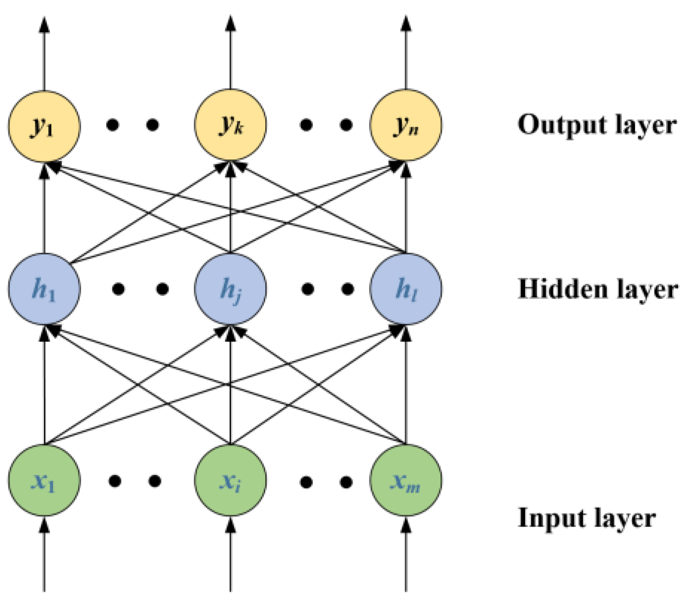
2.3. Extreme Learning Machine
To solve the problem of the slow learning speed of traditional feed forward neural networks, Huang et al. [
28] proposed a new learning algorithm, which is called the ELM. The structure of the ELM is the same as the traditional single hidden layer neural network, as shown in
Figure 4.
In
Figure 4, the input layer of the ELM contains
m neurons, the hidden layer has
l neurons, and the output layer contains
n neurons.
Let
and
denote the connection weight and bias of the input layer and hidden layer. The output
of the neural network is given by
where
g(
x) is the activation function,
is the output weight.
If there are
Q arbitrary samples, the input matrix
X and output matrix
Y are expressed by
If the output matrix of the hidden layer is defined as
H, then
H can be given by
Similarly,
can be expressed by
From Equation (22) to Equation (25), Equation (26) can be derived:
Let
denote an arbitrary sample, where the goal of the ELM is to minimize the output error, which is given by
Equation (27) can be transformed into
By solving the least squares solution of Equation (28), the output weight
can be determined by
where
is the Moore–Penrose generalized inverse of the matrix
H.


