Author Contributions
Conceptualization, L.Z. and F.M.; methodology, L.Z.; software, Z.L.; validation, J.Z., Z.L. and T.W.; formal analysis, J.Z.; investigation, J.Z.; resources, Z.L.; data curation, Z.L.; writing—original draft preparation, L.Z.; writing—review and editing, Ma fang; visualization, T.W.; supervision, C.L.; funding acquisition, F.M., L.Z.
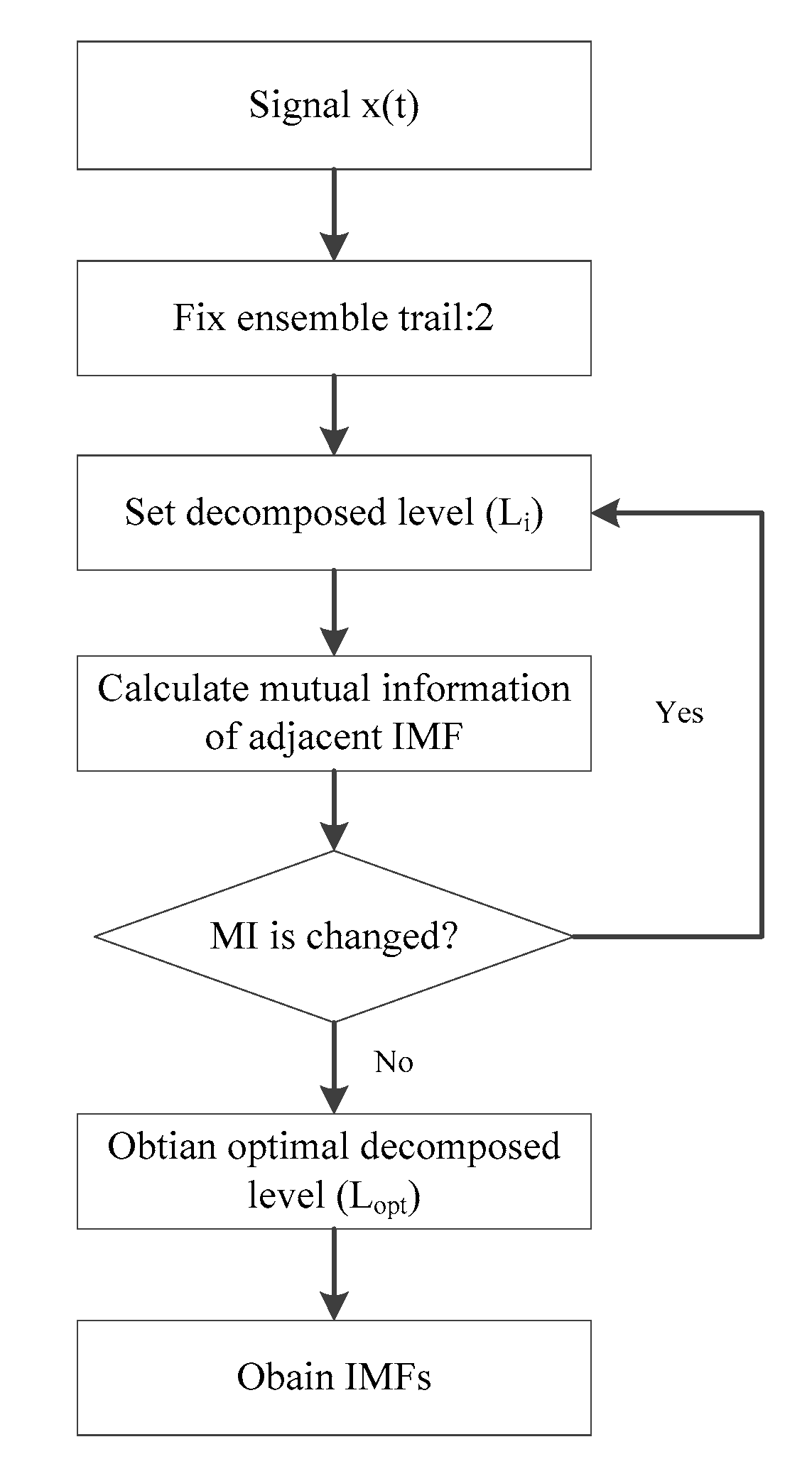
Figure 1.
Flowchart of enhanced complementary empirical mode decomposition with adaptive noise (ECEEMDAN).
Figure 1.
Flowchart of enhanced complementary empirical mode decomposition with adaptive noise (ECEEMDAN).
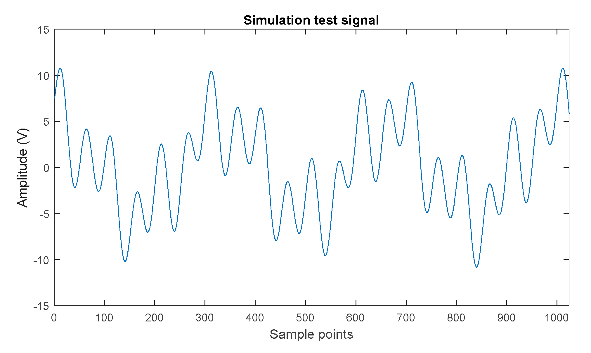
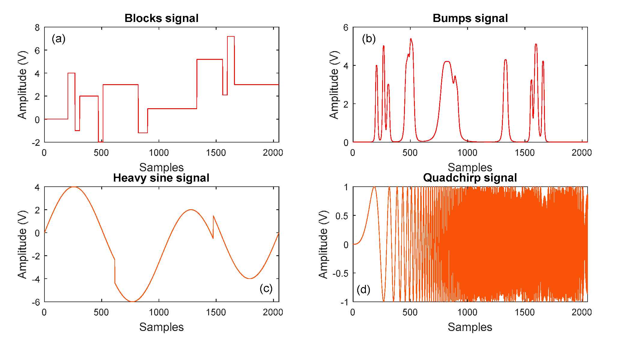
Figure 2.
Test simulation signal with the specified frequency component.
Figure 2.
Test simulation signal with the specified frequency component.
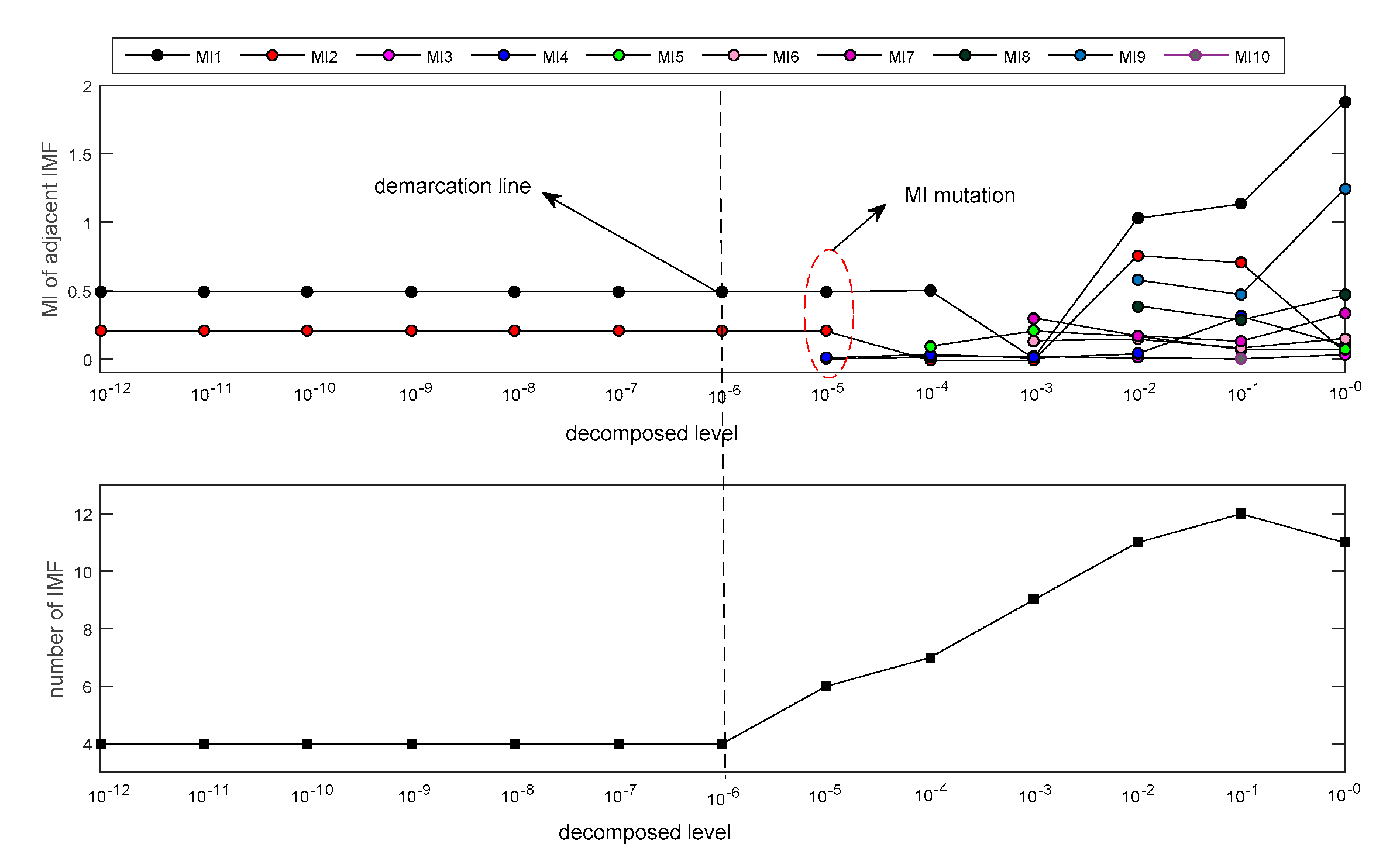
Figure 3.
Decomposition results for the simulation signal (SSC) signal under different decomposition levels.
Figure 3.
Decomposition results for the simulation signal (SSC) signal under different decomposition levels.
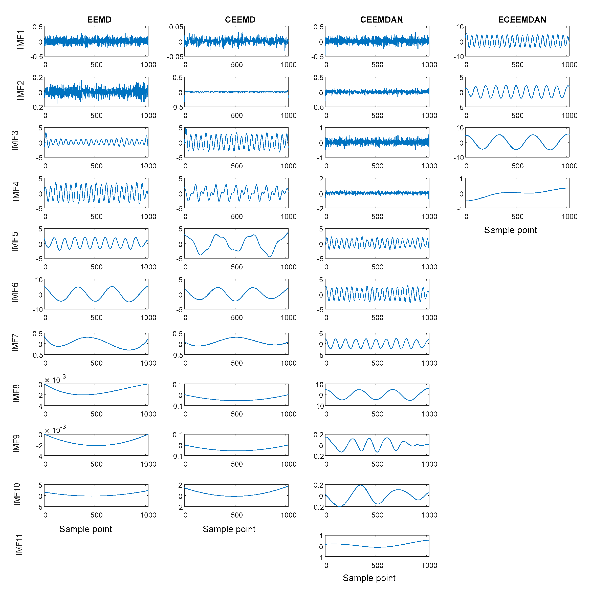
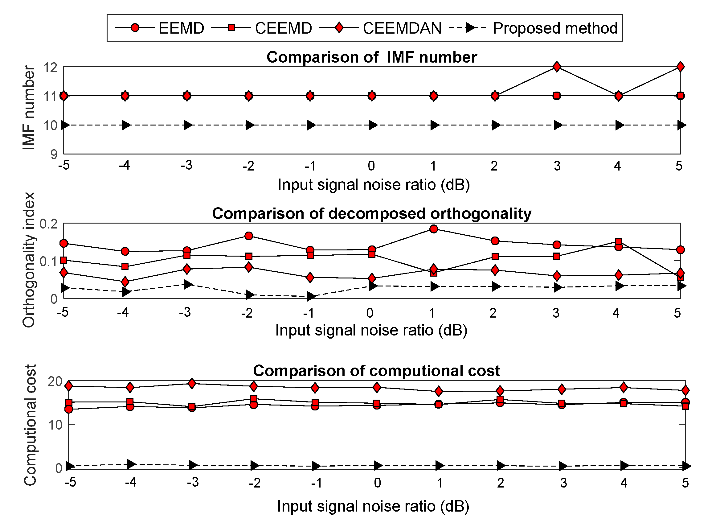
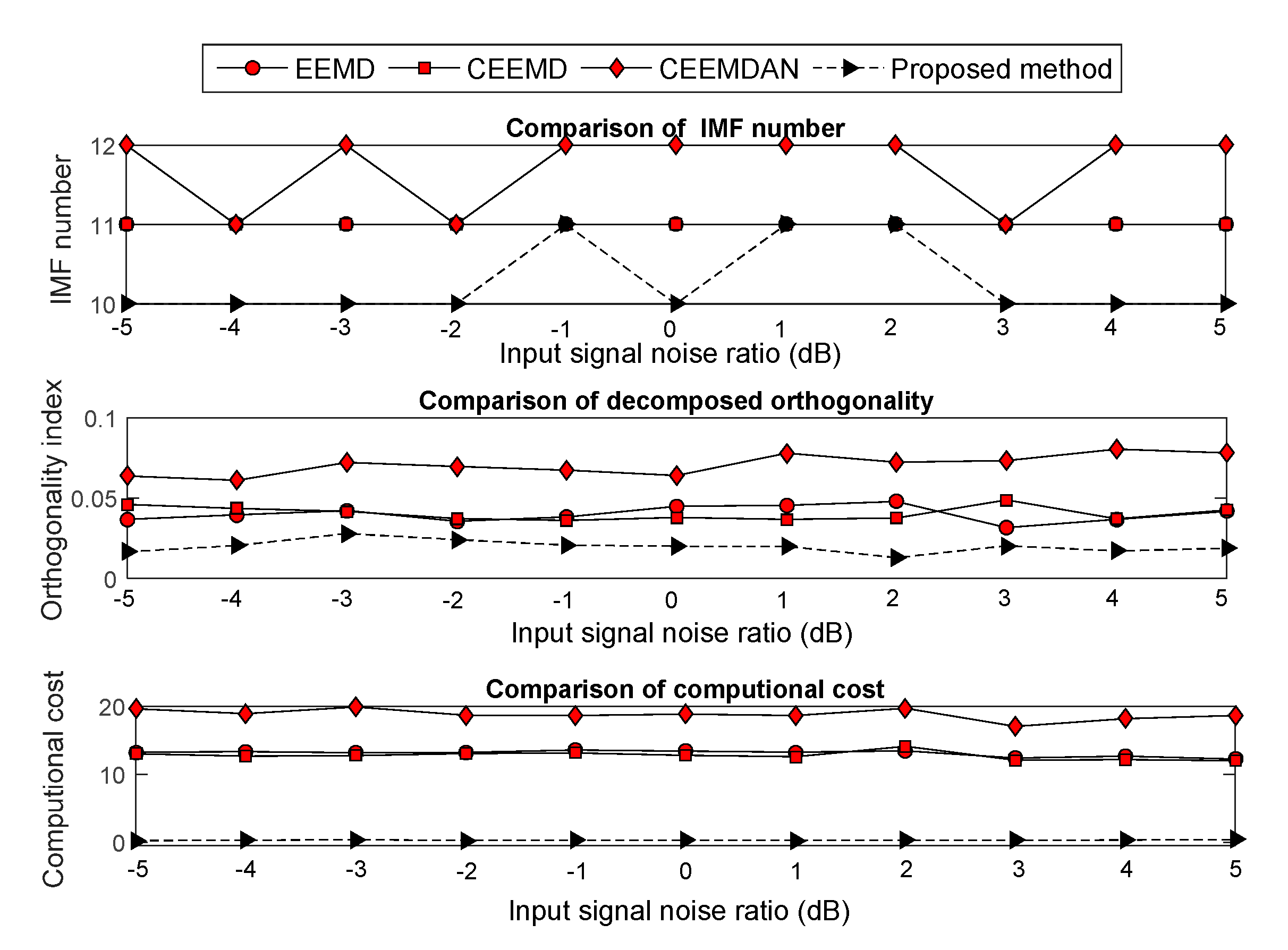
Figure 4.
Comparison of decomposing effects of empirical mode decomposition (EMD) improved versions with ECEEMDAN.
Figure 4.
Comparison of decomposing effects of empirical mode decomposition (EMD) improved versions with ECEEMDAN.
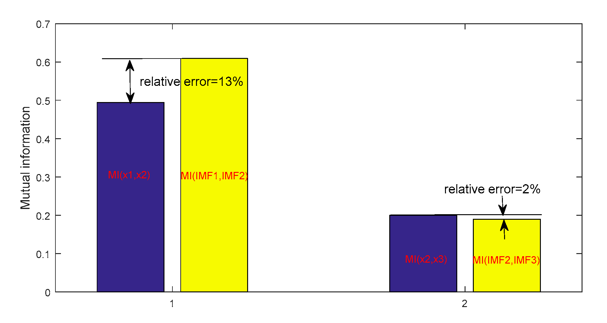
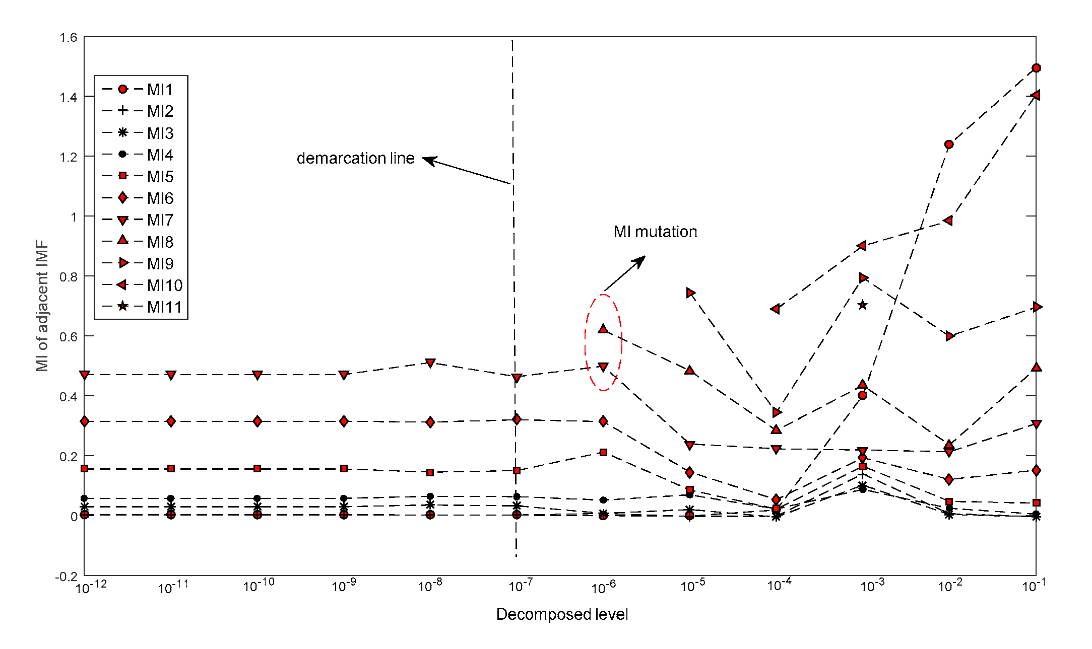
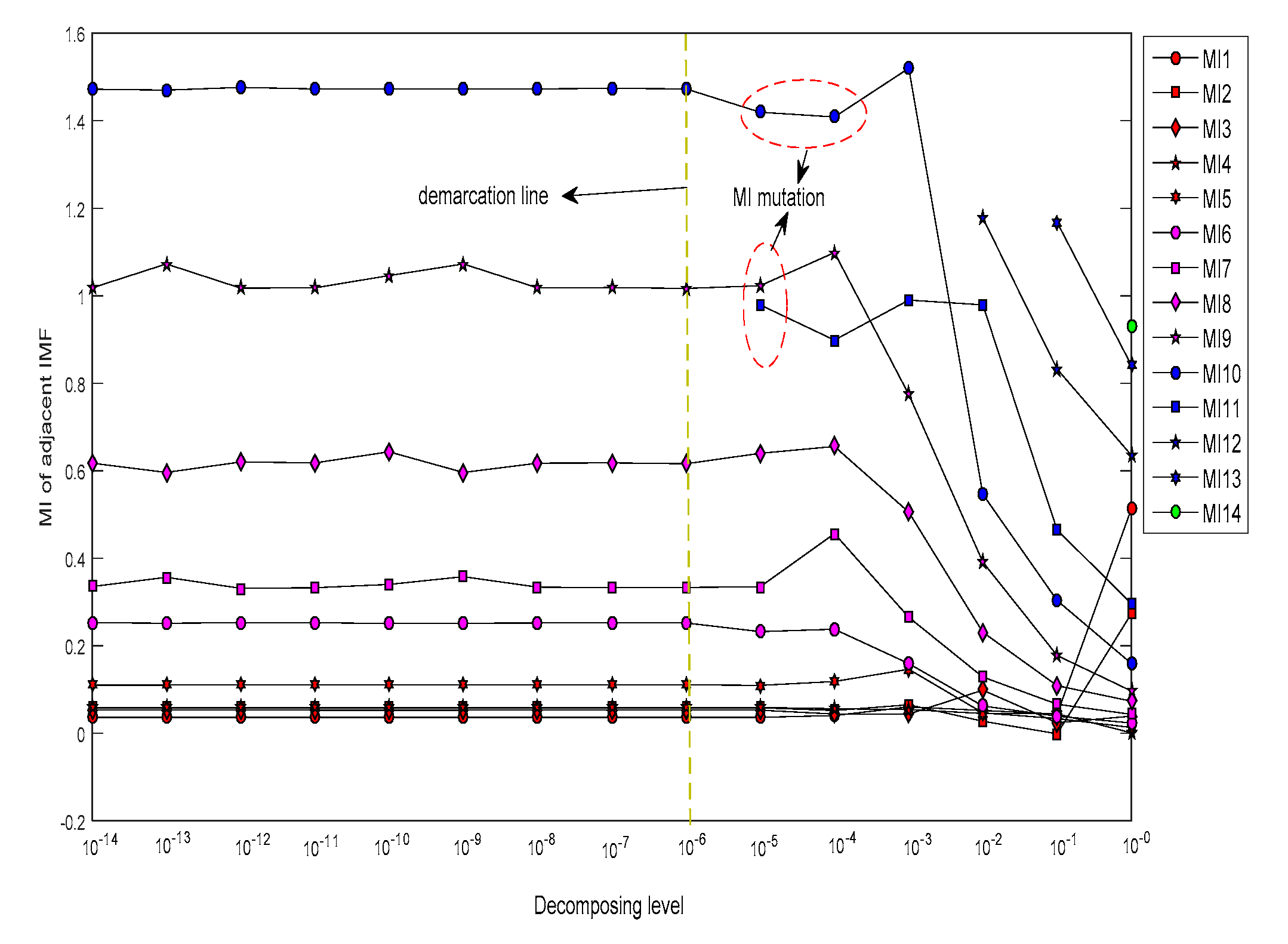
Figure 5.
Mutual information (MI) comparison of information component of original signal and corresponding intrinsic mode functions (IMFs).
Figure 5.
Mutual information (MI) comparison of information component of original signal and corresponding intrinsic mode functions (IMFs).
Figure 6.
Simulation of the noisy signal.
Figure 6.
Simulation of the noisy signal.
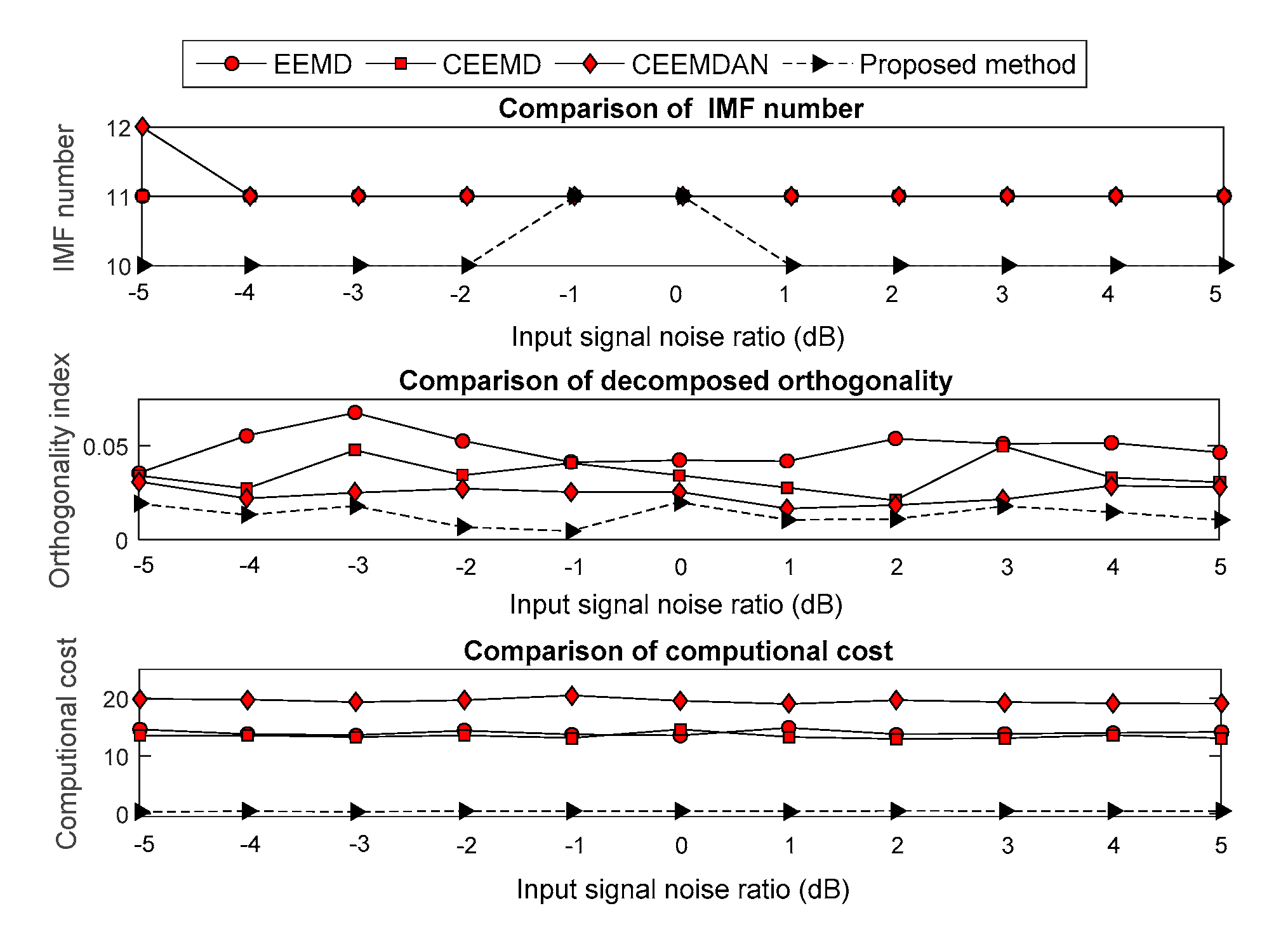
Figure 7.
Comparison of the decomposition effect for the ‘blocks’ signal.
Figure 7.
Comparison of the decomposition effect for the ‘blocks’ signal.
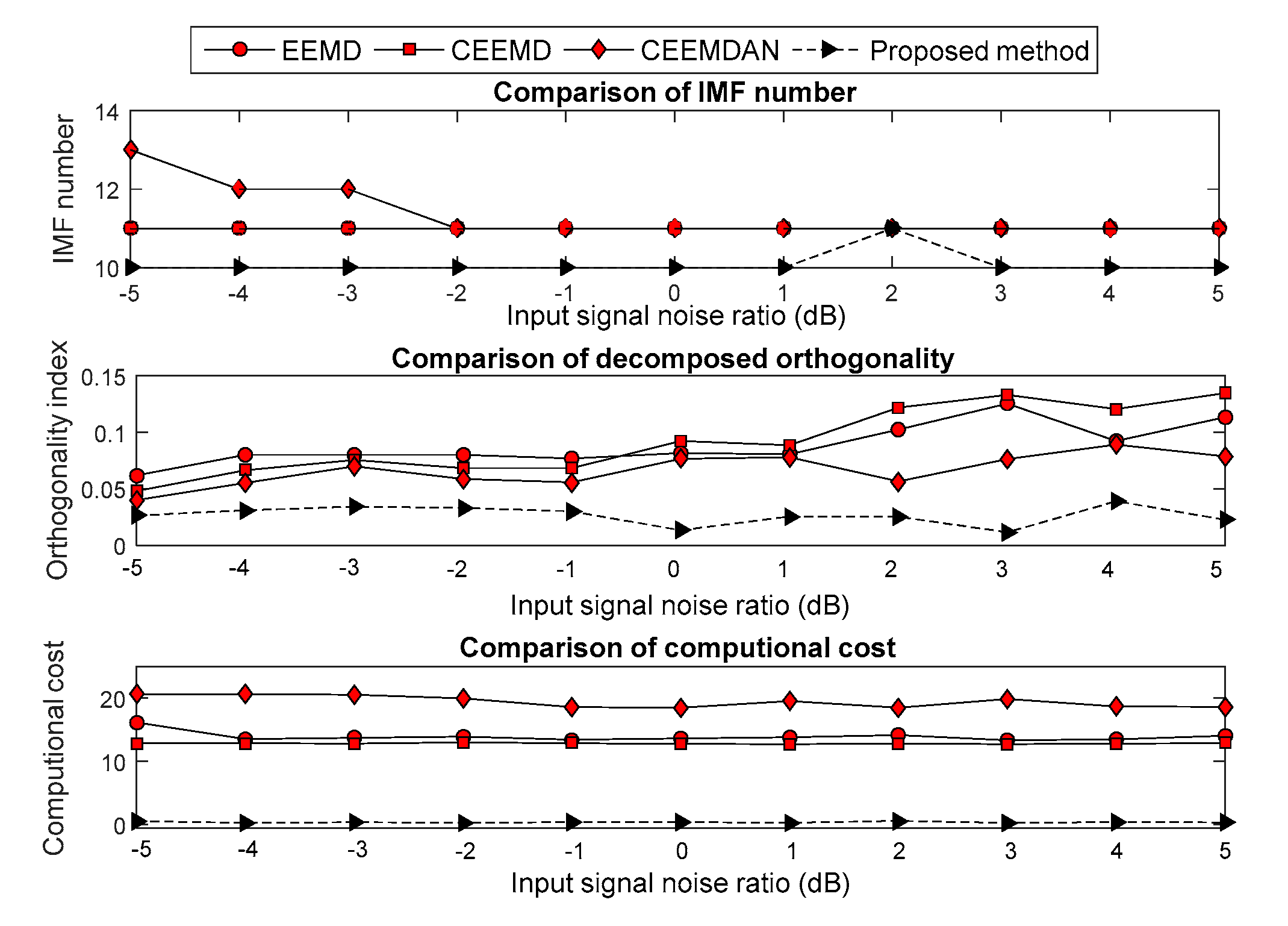
Figure 8.
Comparison of the decomposition effect for the ‘bumps’ signal.
Figure 8.
Comparison of the decomposition effect for the ‘bumps’ signal.
Figure 9.
Comparison of the decomposition effect for the ‘heavy sine wave’ signal.
Figure 9.
Comparison of the decomposition effect for the ‘heavy sine wave’ signal.
Figure 10.
Comparison of the decomposition effect for the ‘quadchirp’ signal.
Figure 10.
Comparison of the decomposition effect for the ‘quadchirp’ signal.
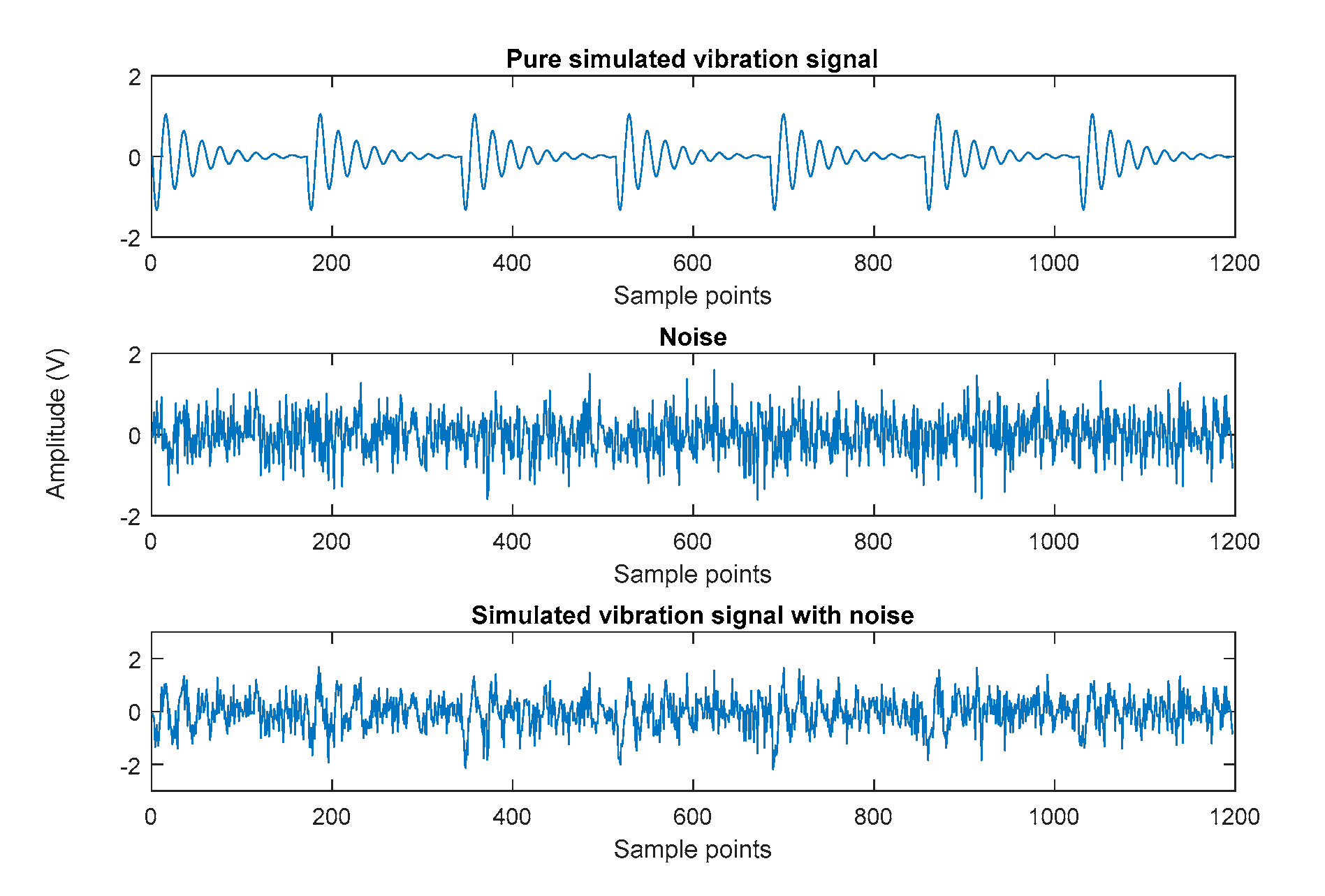
Figure 11.
Simulated vibration signal.
Figure 11.
Simulated vibration signal.
Figure 12.
Decomposition result for simulated vibration signal (SVS) signal under different decomposing level.
Figure 12.
Decomposition result for simulated vibration signal (SVS) signal under different decomposing level.
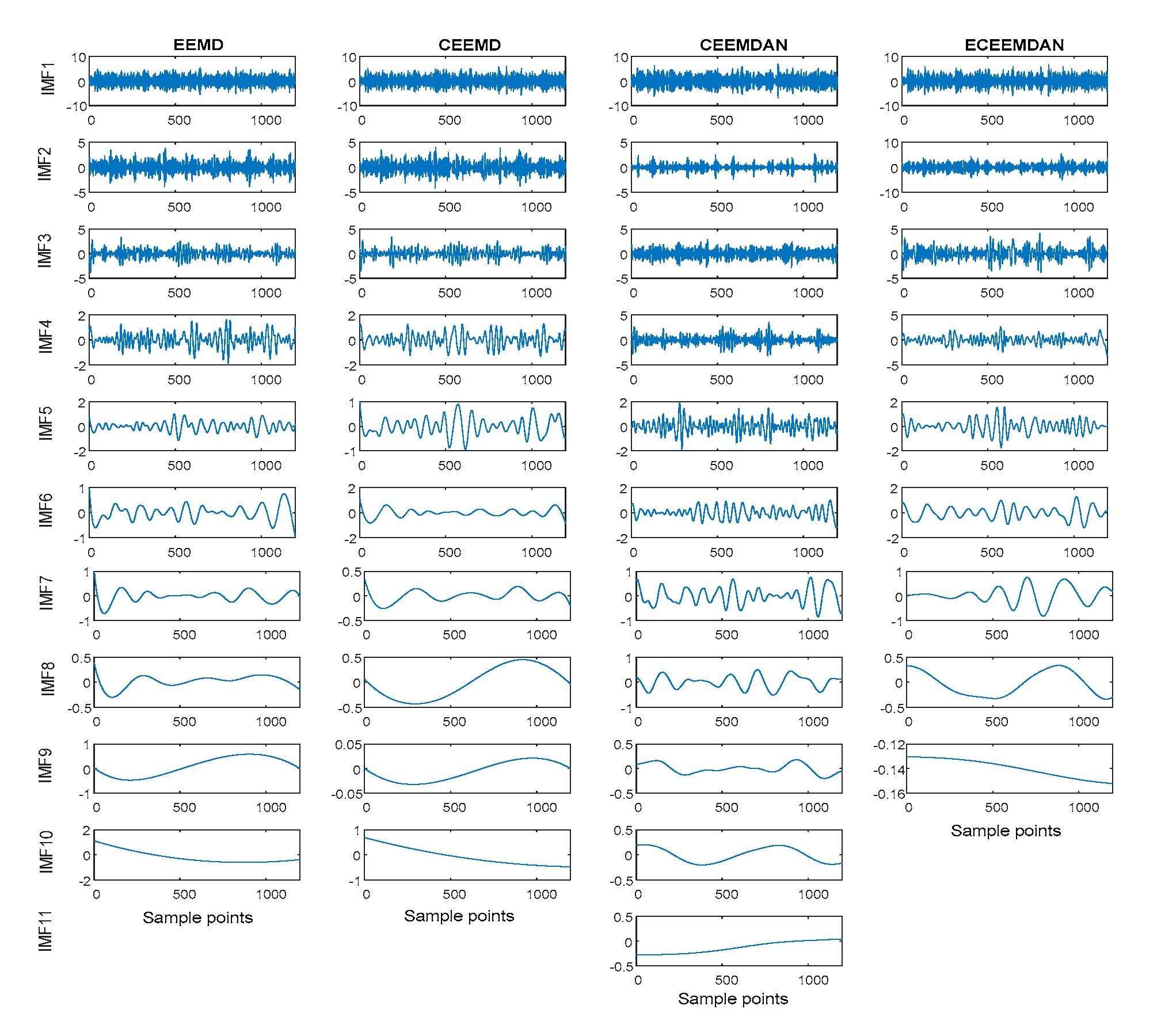
Figure 13.
Decomposing result of SVS signal with the improved EMD versions and ECEEMDAN.
Figure 13.
Decomposing result of SVS signal with the improved EMD versions and ECEEMDAN.
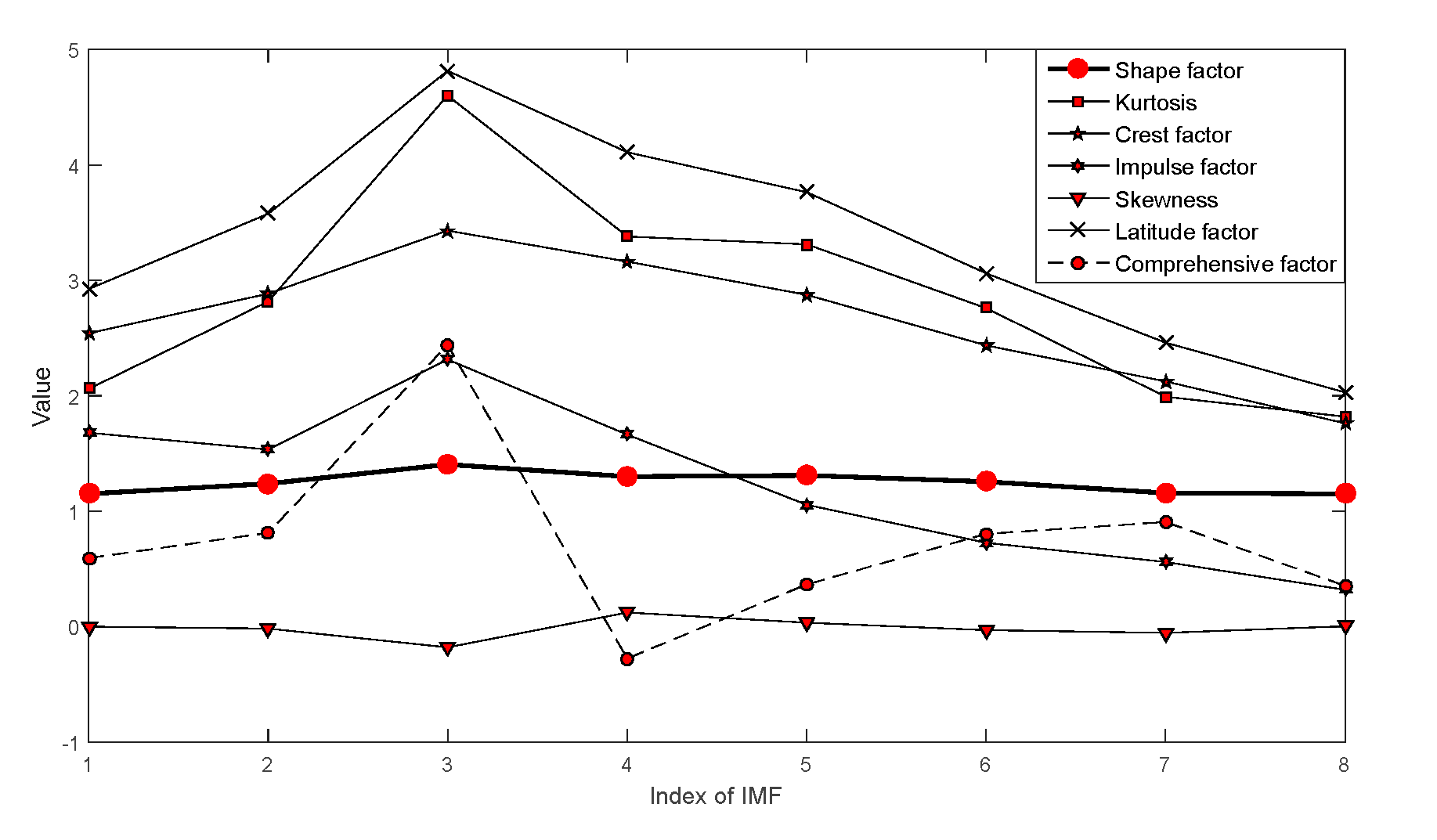
Figure 14.
Comprehensive factor and factor of single statistical method.
Figure 14.
Comprehensive factor and factor of single statistical method.
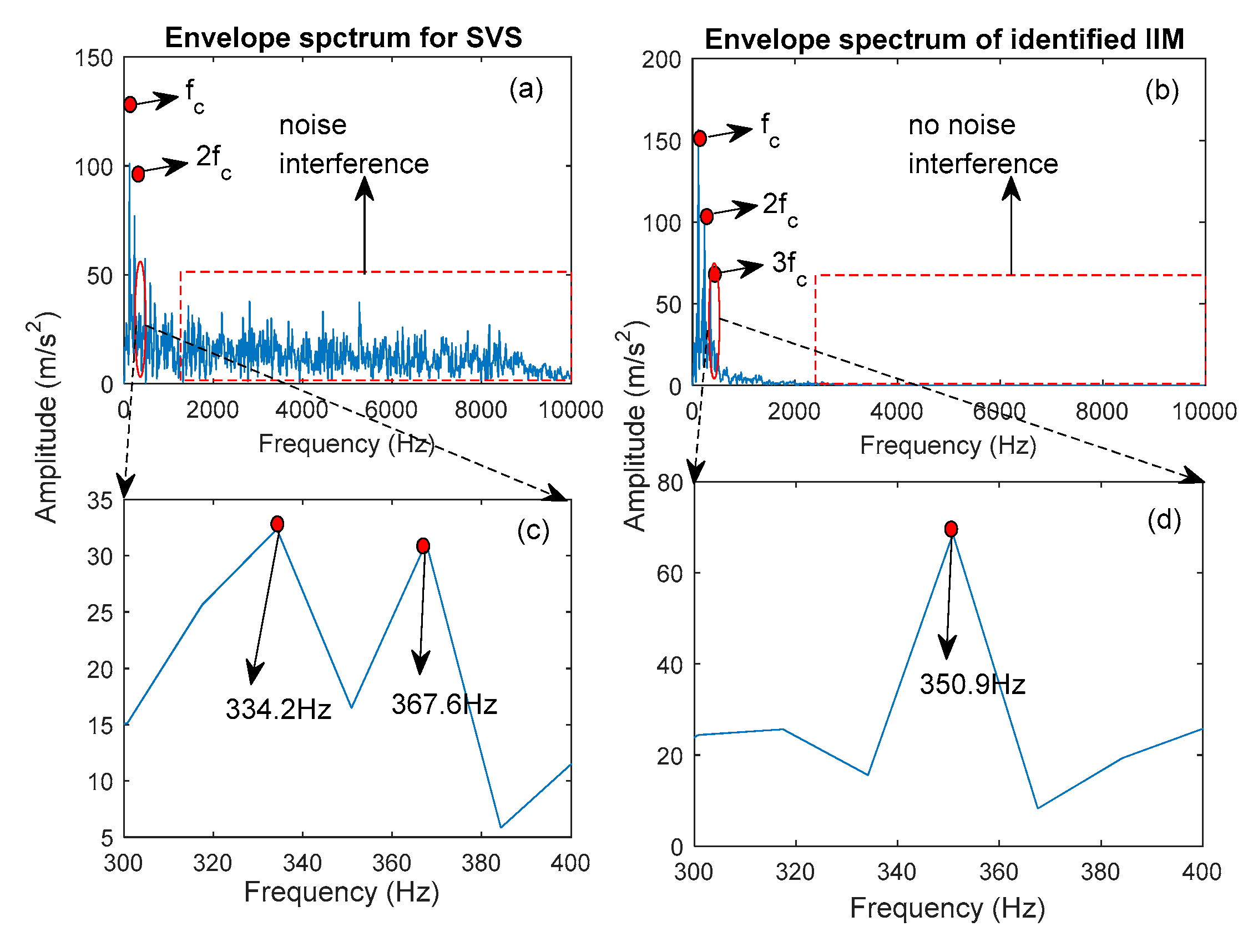
Figure 15.
Comparison of fault frequency identification for the SVS signal and IIM. (a,b) the identified result of the feature frequency; (c,d) comprehensively shows the identified result.
Figure 15.
Comparison of fault frequency identification for the SVS signal and IIM. (a,b) the identified result of the feature frequency; (c,d) comprehensively shows the identified result.
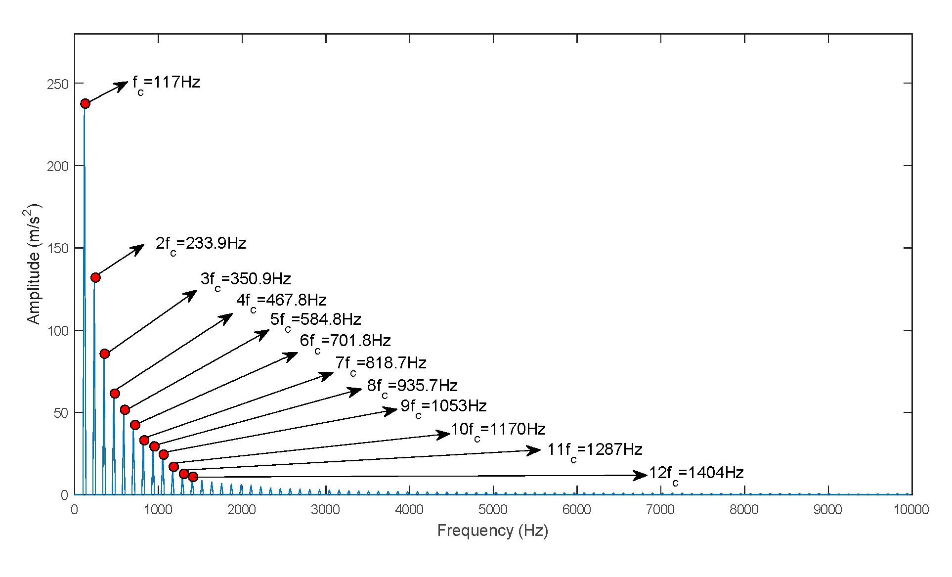
Figure 16.
Octave frequency of the real signal.
Figure 16.
Octave frequency of the real signal.
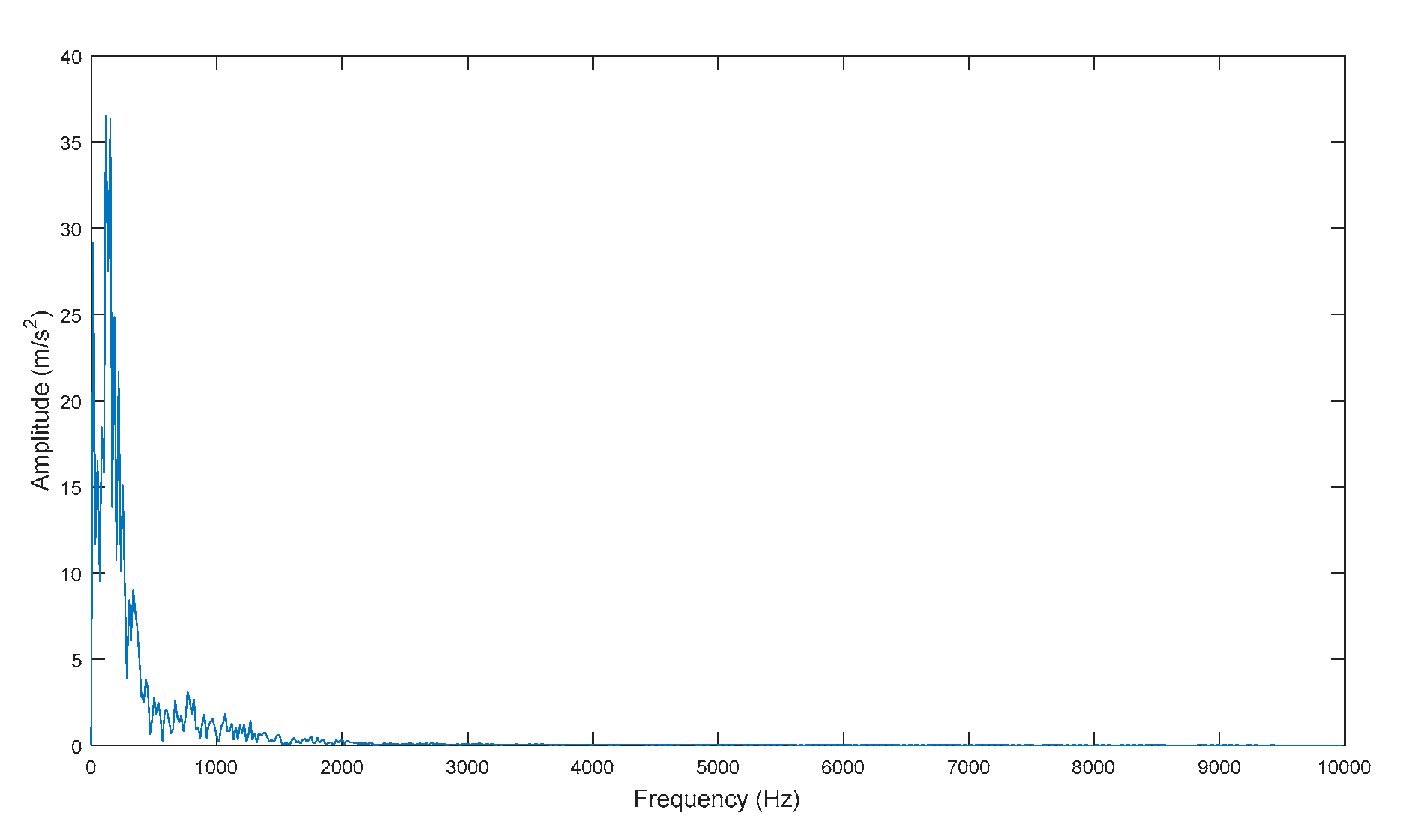
Figure 17.
Envelope spectrum of the fourth IMF (IMF4).
Figure 17.
Envelope spectrum of the fourth IMF (IMF4).
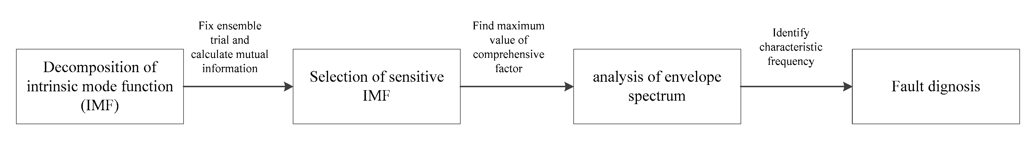
Figure 18.
Flowchart of fault diagnosis.
Figure 18.
Flowchart of fault diagnosis.
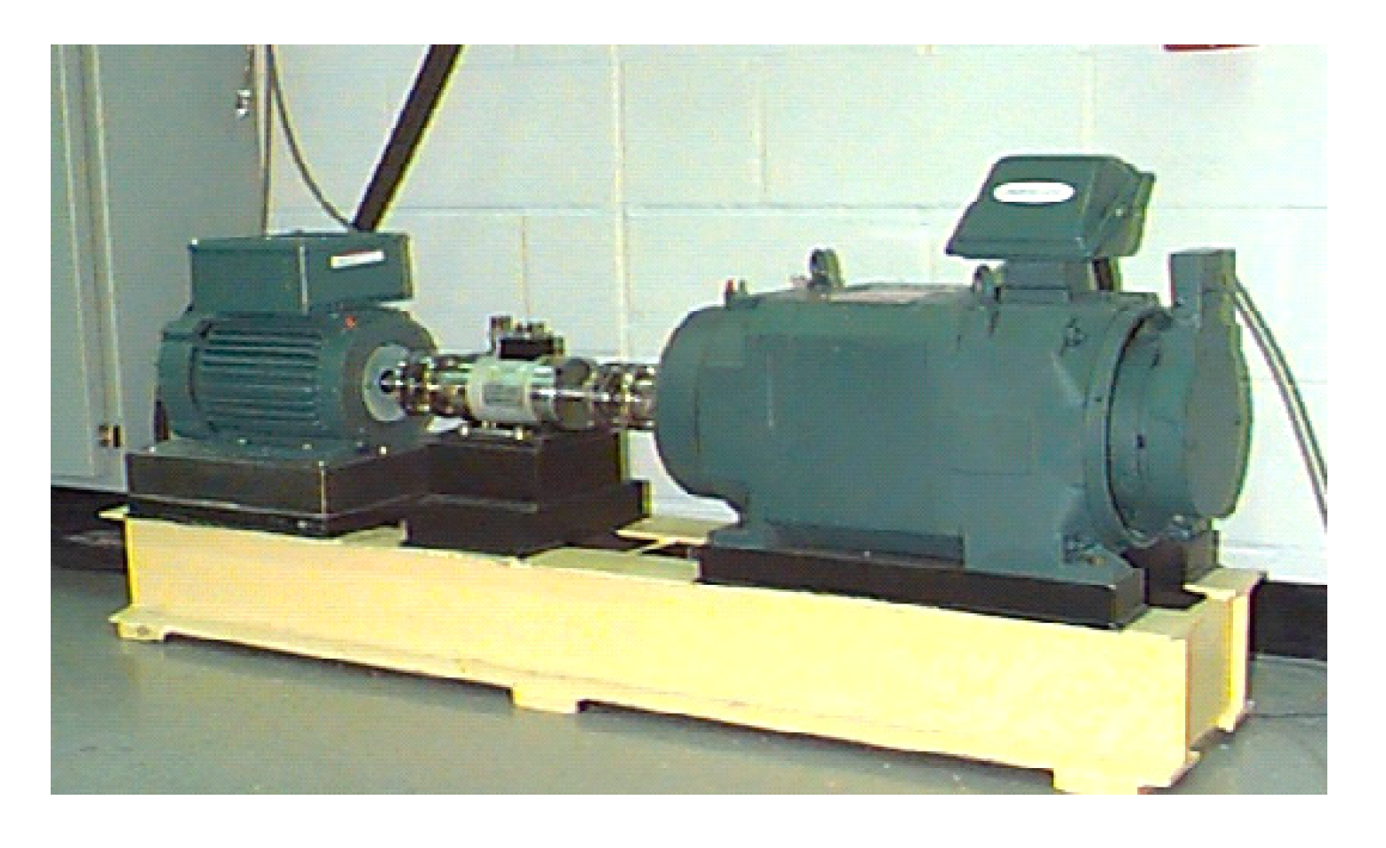
Figure 19.
Test rig from the Case Western Reserve University.
Figure 19.
Test rig from the Case Western Reserve University.
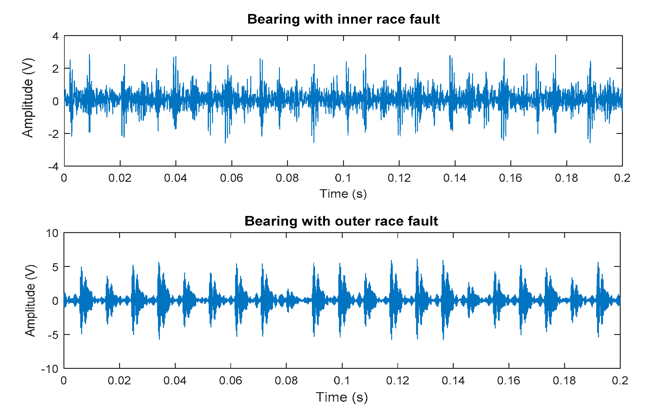
Figure 20.
Experimental data of inner and outer raceway fault.
Figure 20.
Experimental data of inner and outer raceway fault.
Figure 21.
Decomposition result for a vibration signal with an inner raceway fault.
Figure 21.
Decomposition result for a vibration signal with an inner raceway fault.
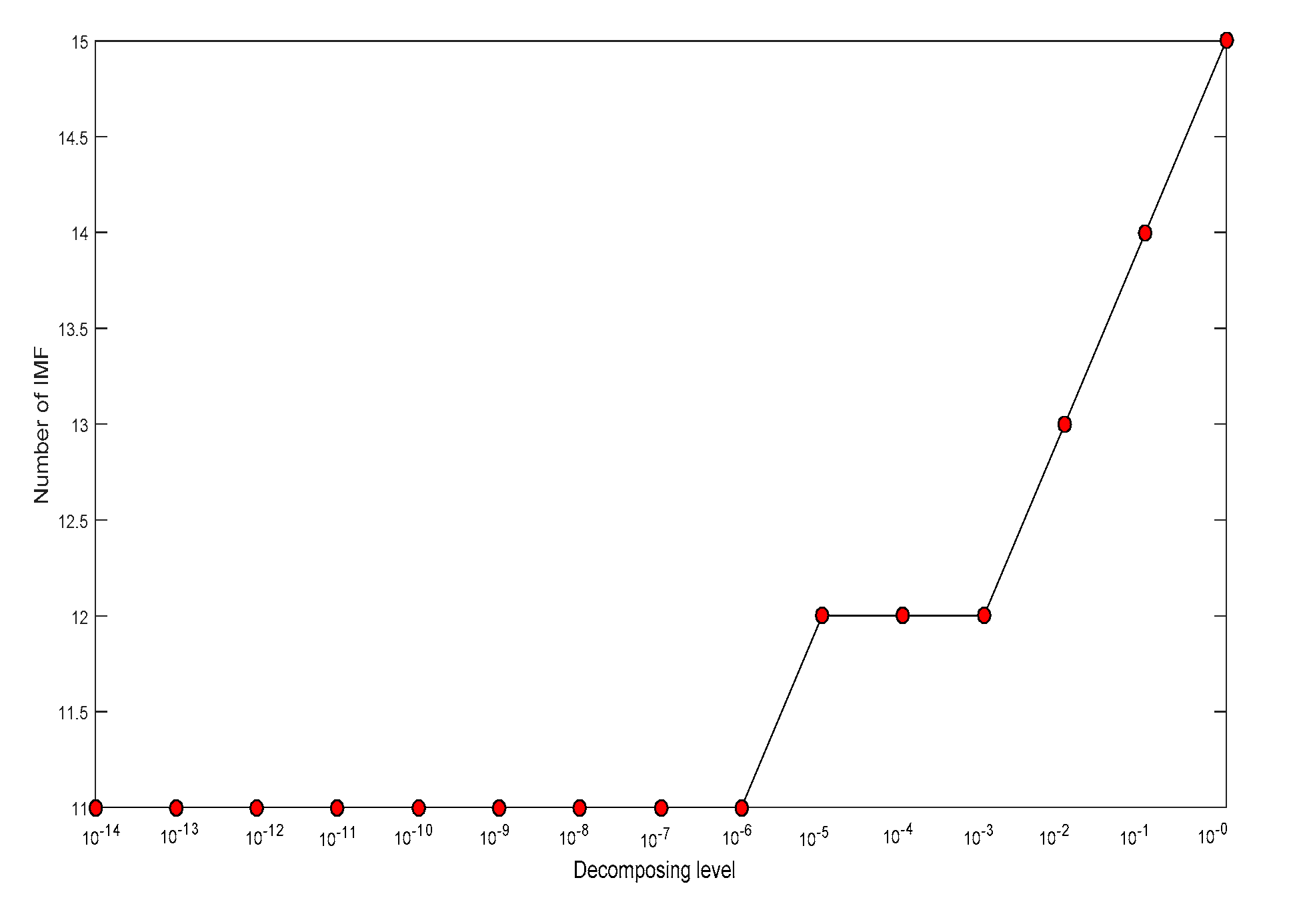
Figure 22.
Decomposition number corresponding to each decomposition level.
Figure 22.
Decomposition number corresponding to each decomposition level.
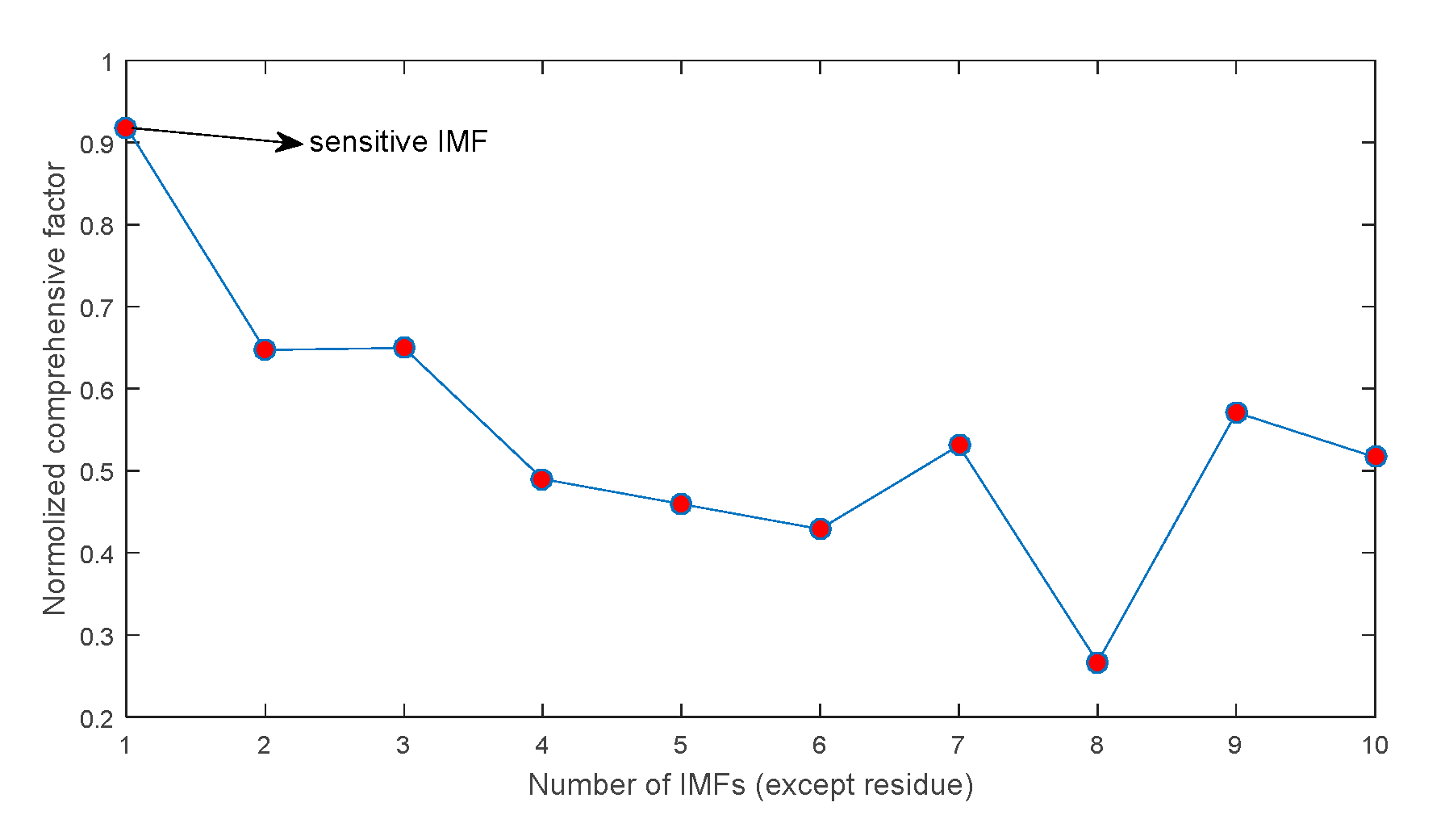
Figure 23.
CF of each IMF.
Figure 23.
CF of each IMF.
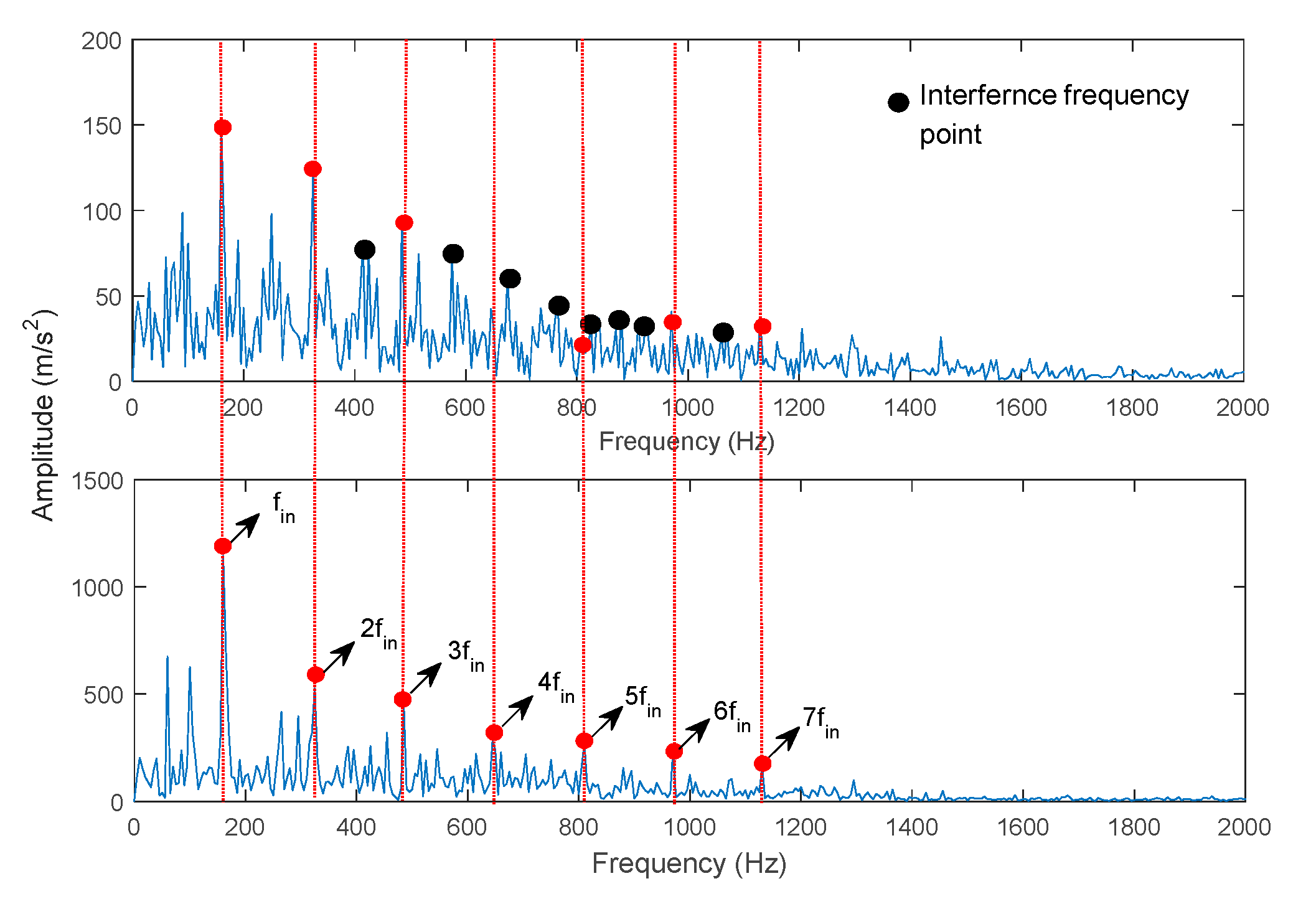
Figure 24.
Comparison of extraction fault frequency for ECEEMDAN and CEEMDAN.
Figure 24.
Comparison of extraction fault frequency for ECEEMDAN and CEEMDAN.
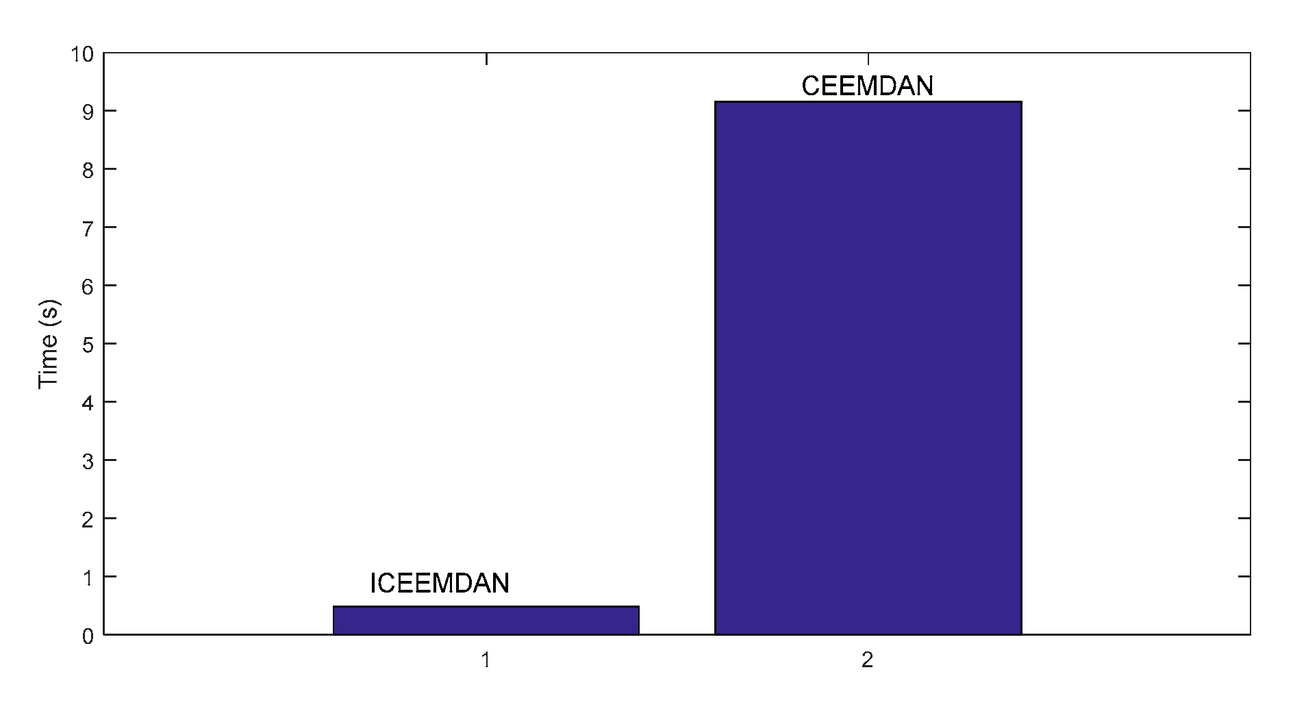
Figure 25.
Comparison of computational cost for ECEEMDAN and CEEMDAN.
Figure 25.
Comparison of computational cost for ECEEMDAN and CEEMDAN.
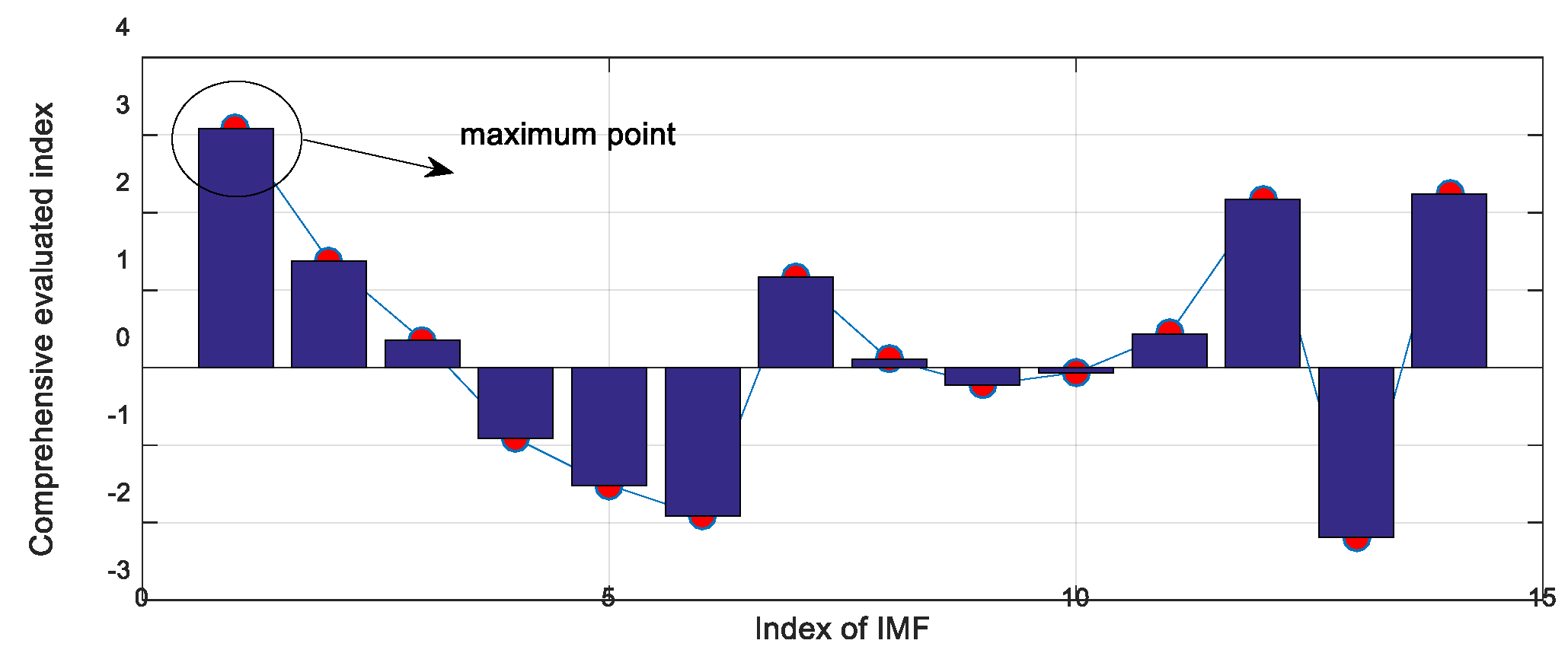
Figure 26.
Selection of IIM with (ECEEMDAN-CF).
Figure 26.
Selection of IIM with (ECEEMDAN-CF).
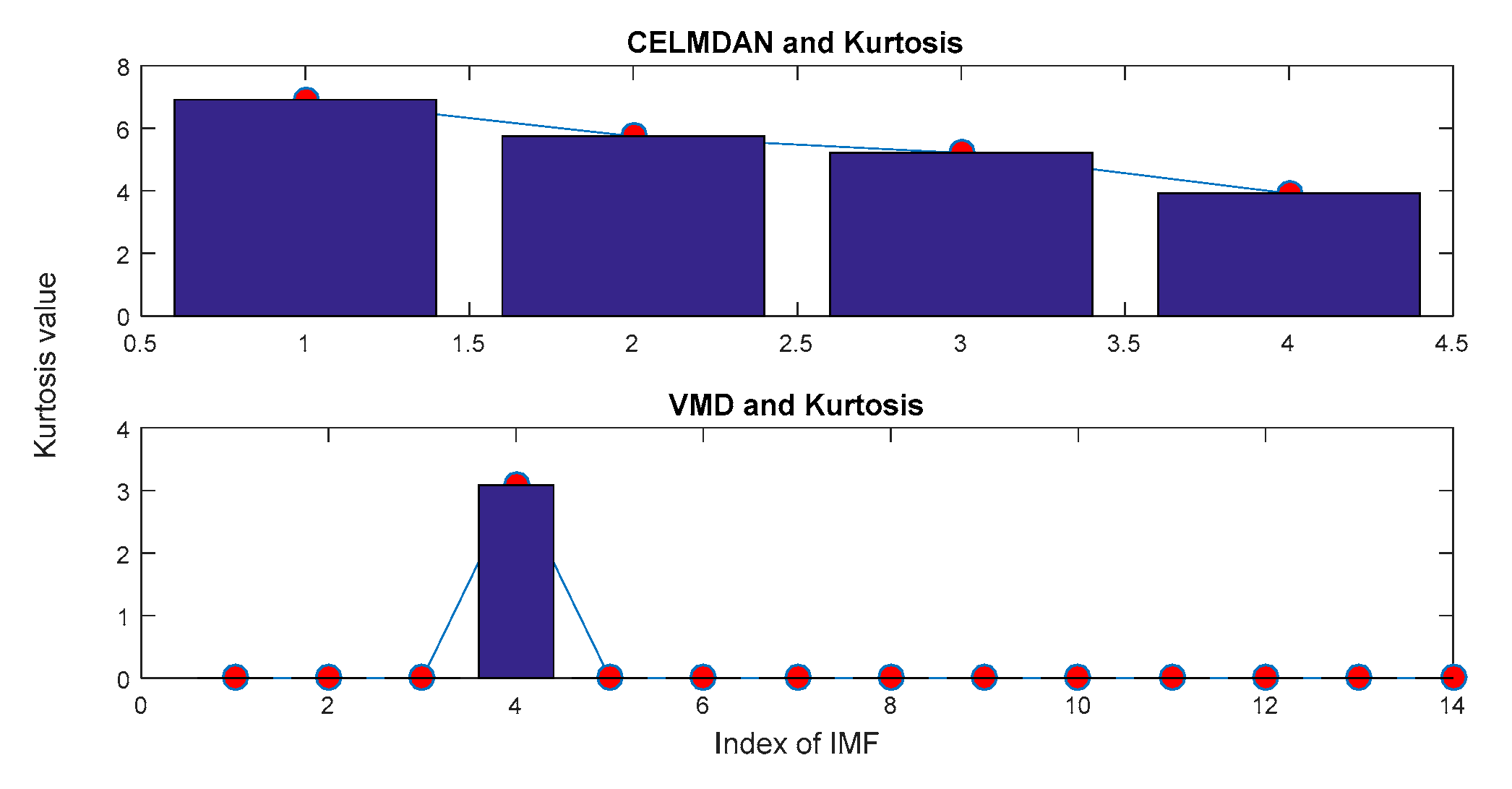
Figure 27.
Selection of IIM with CELMDAN kurtosis and VMD kurtosis.
Figure 27.
Selection of IIM with CELMDAN kurtosis and VMD kurtosis.
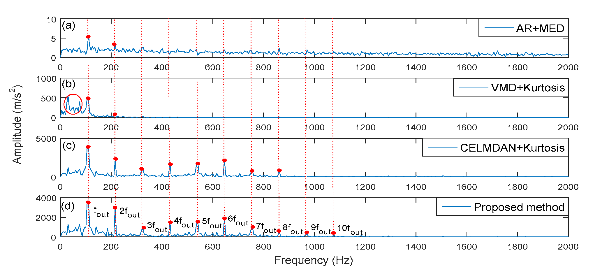
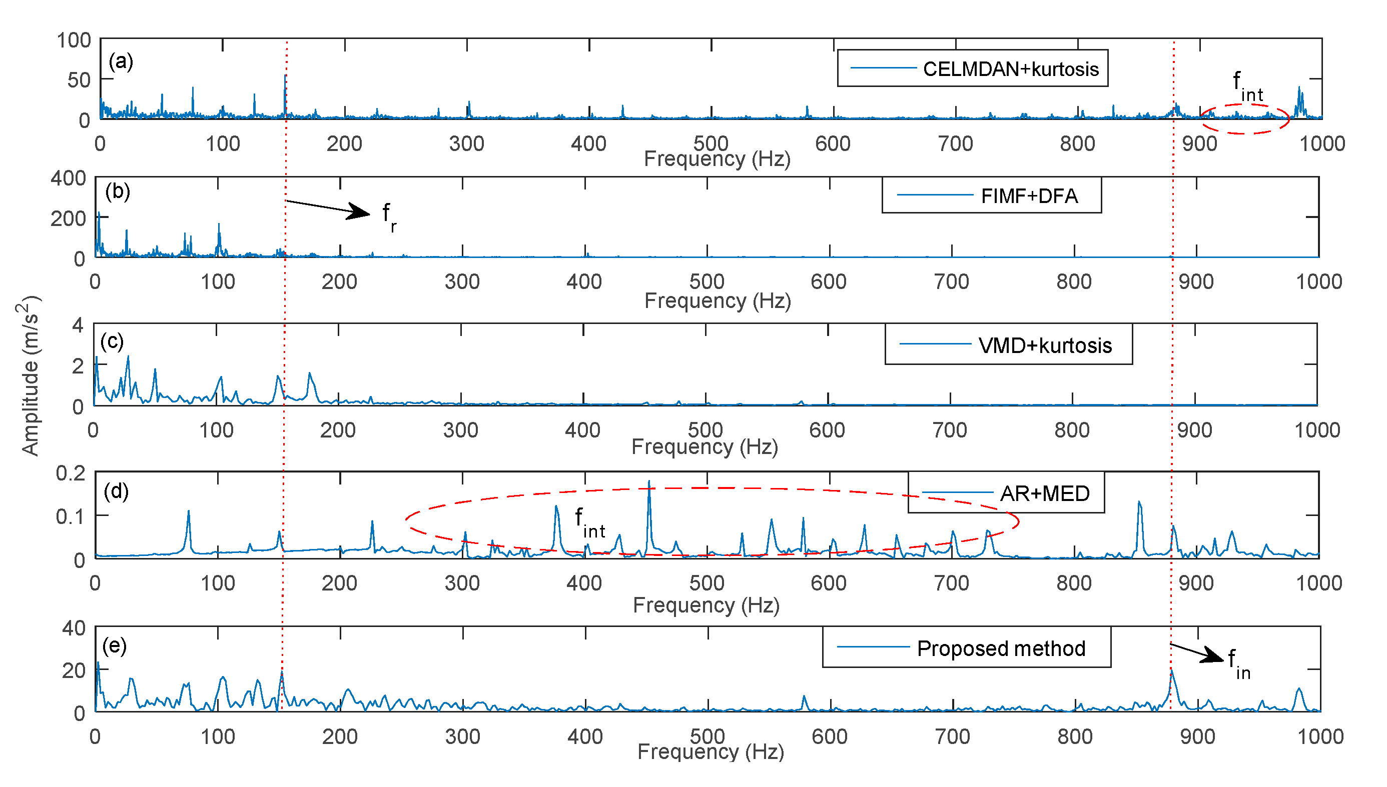
Figure 28.
Comparison of fault extraction using the different methods.
Figure 28.
Comparison of fault extraction using the different methods.
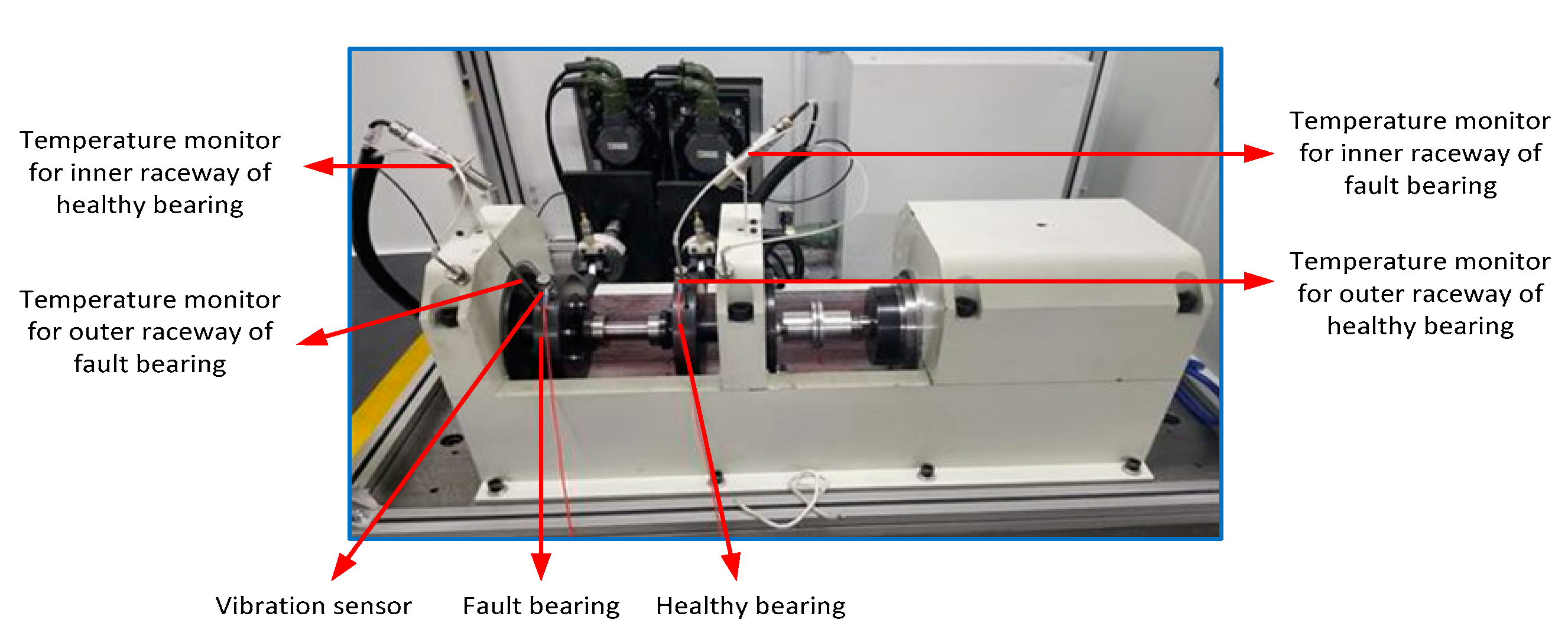
Figure 29.
Experiment rig from real measurement.
Figure 29.
Experiment rig from real measurement.
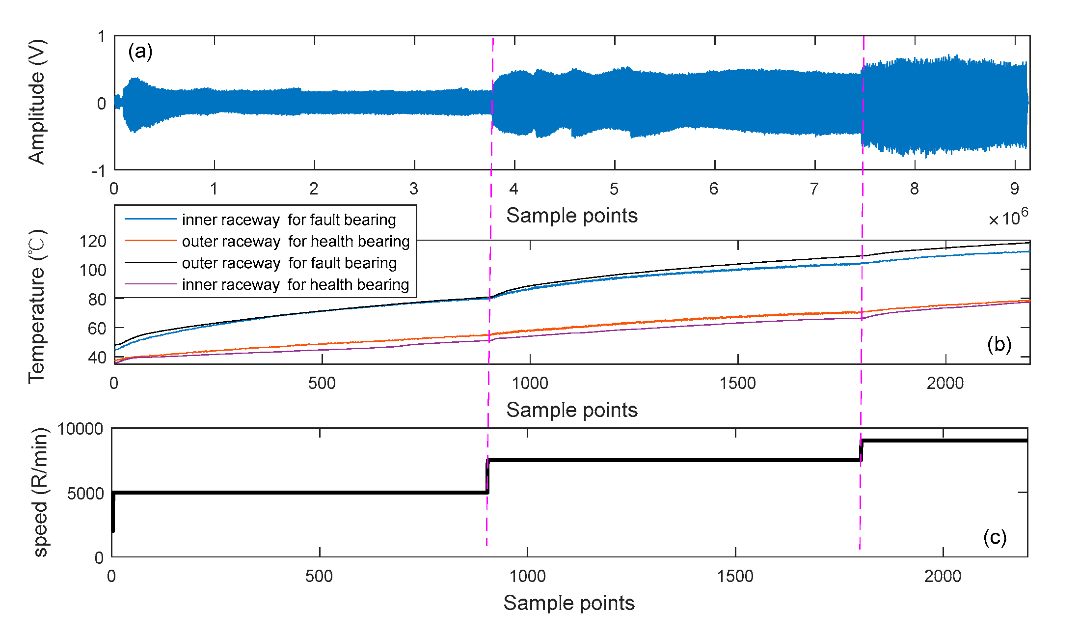
Figure 30.
Monitored data of different test conditions. (a) vibration signal, (b) temperature signal, and (c) rotational speed.
Figure 30.
Monitored data of different test conditions. (a) vibration signal, (b) temperature signal, and (c) rotational speed.
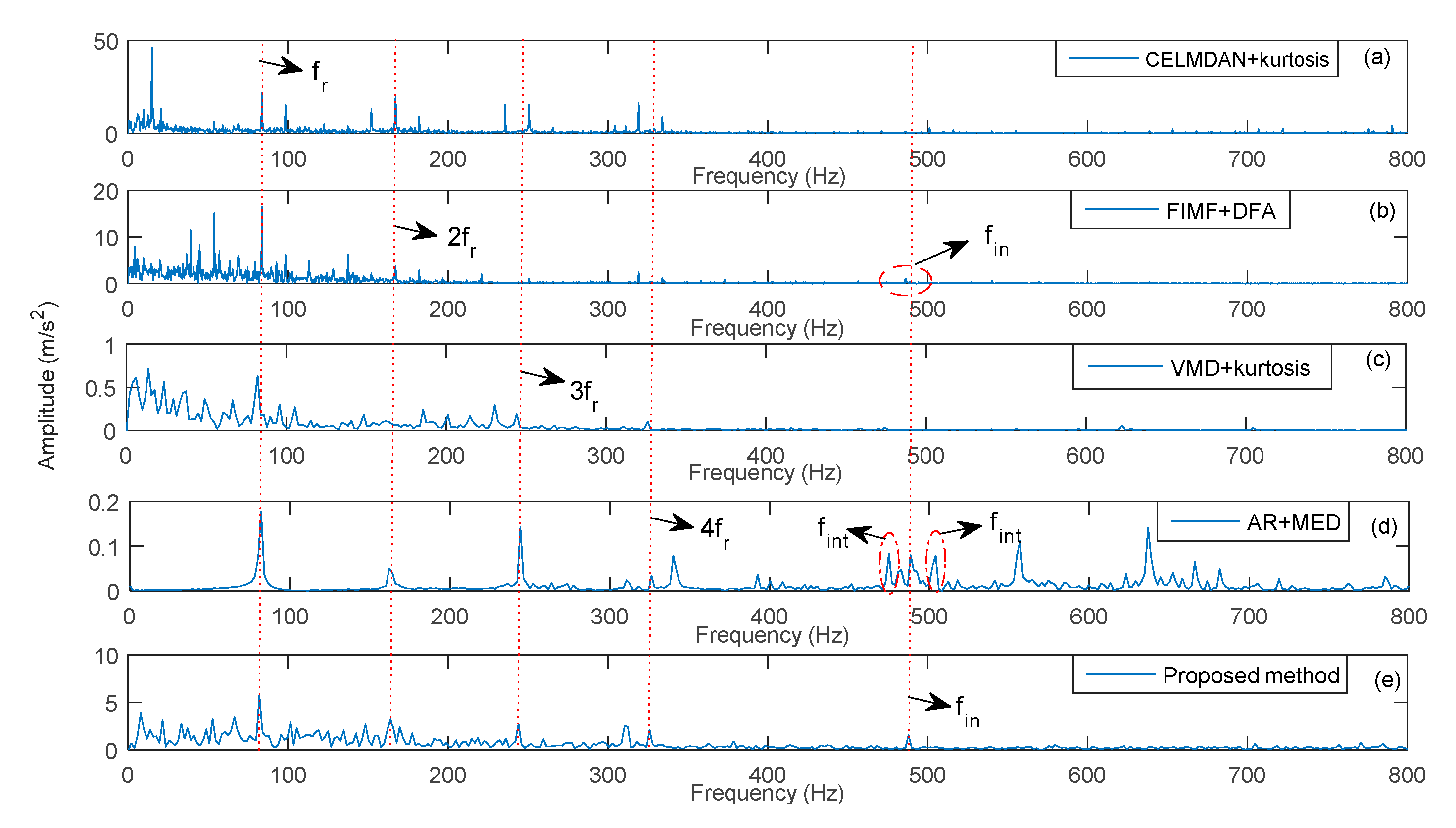
Figure 31.
Identified fault frequency of a rolling bearing at 5000 RPM.
Figure 31.
Identified fault frequency of a rolling bearing at 5000 RPM.
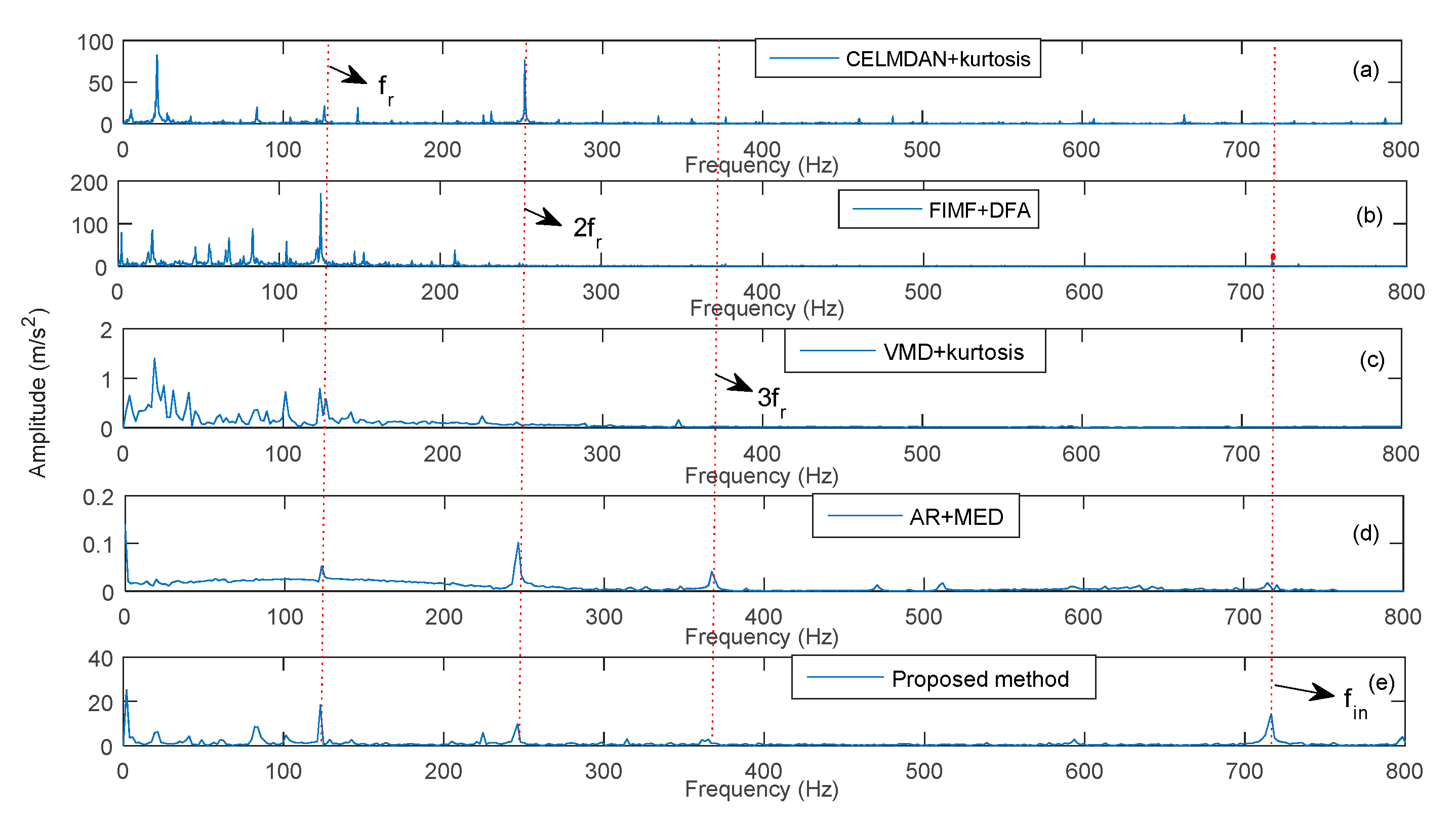
Figure 32.
Identified fault frequency of a rolling bearing at 7500 RPM.
Figure 32.
Identified fault frequency of a rolling bearing at 7500 RPM.
Figure 33.
Identified fault frequency of a rolling bearing at 9000 RPM.
Figure 33.
Identified fault frequency of a rolling bearing at 9000 RPM.
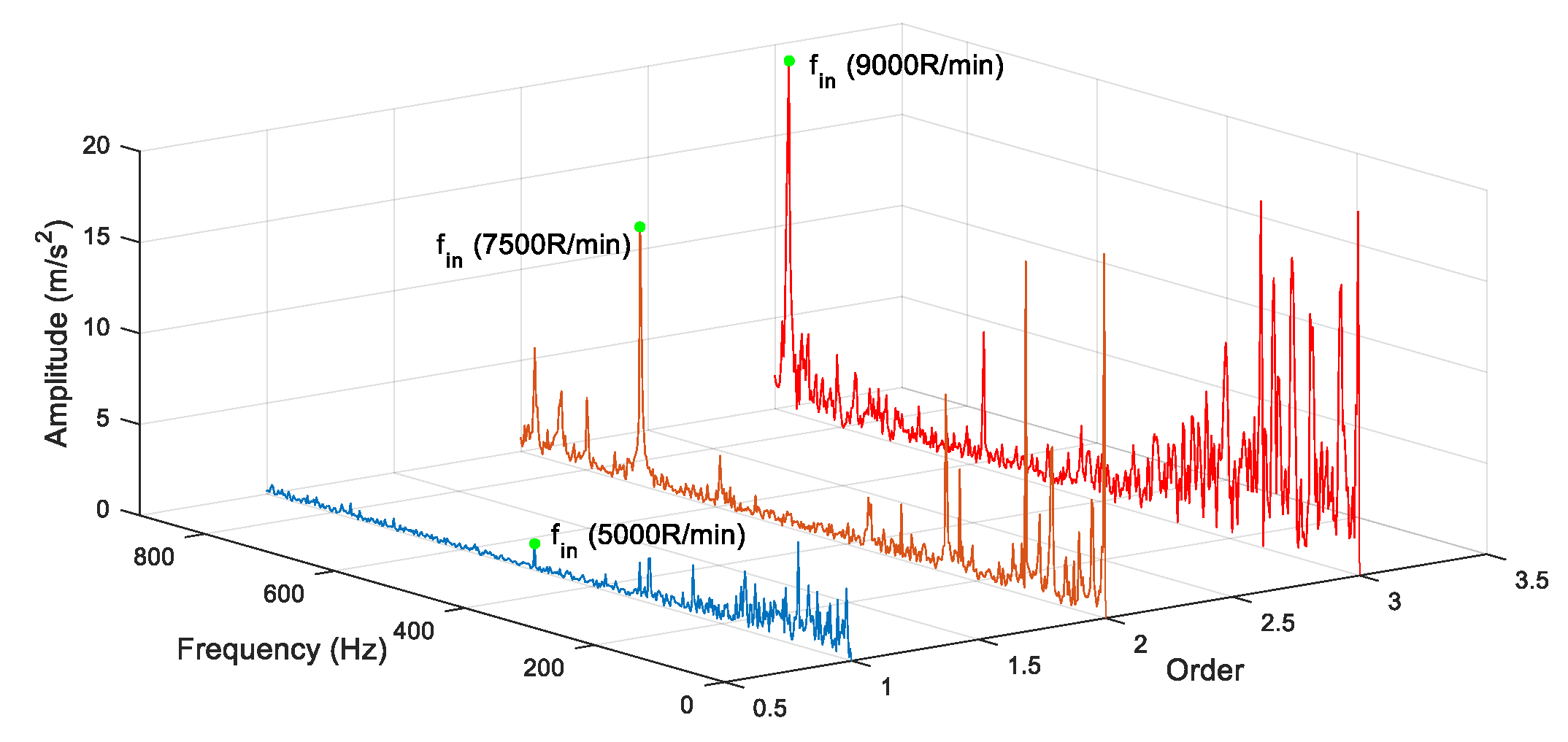
Figure 34.
Comparison of feature frequency at different rotation speed.
Figure 34.
Comparison of feature frequency at different rotation speed.
Table 1.
Comparison of the decomposition effect.
Table 1.
Comparison of the decomposition effect.
| Method | Number of IMF | Computation Time (s) | Orthogonality Index |
|---|
| EEMD | 10 | 7.88 | 0.11 |
| CEEMD | 10 | 7.58 | 0.20 |
| CEEMDAN | 11 | 10.16 | 0.10 |
| ECEEMDAN | 4 | 0.09 | 0.03 |
Table 2.
Decomposition number of the IMF under each decomposition level.
Table 2.
Decomposition number of the IMF under each decomposition level.
| Decomposition Level (L) |
|---|
| 10−12 | 10−11 | 10−10 | 10−9 | 10−8 | 10−7 | 10−6 | 10−5 | 10−4 | 10−3 | 10−2 | 10−1 |
|---|
| IMF number | 9 | 9 | 9 | 9 | 9 | 9 | 10 | 11 | 12 | 13 | 12 | 12 |
Table 3.
Comparison of decomposition effect for the simulation signal.
Table 3.
Comparison of decomposition effect for the simulation signal.
| Method | Number of IMF | Computation Time (s) | Orthogonality Index |
|---|
| EEMD | 10 | 17.83 | 0.15 |
| CEEMD | 10 | 16.59 | 0.14 |
| CEEMDAN | 11 | 25.89 | 0.12 |
| ECEEMDAN | 9 | 1.01 | 0.07 |
Table 4.
Statistical methods of IIM selection.
Table 4.
Statistical methods of IIM selection.
| Number | Statistical Parameter | Expression |
|---|
| 1 | Shape factor | |
| 2 | Crest factor | |
| 3 | Impulse factor | |
| 4 | Kurtosis | |
| 5 | Skewness | |
| 6 | Latitude factor | |
Table 5.
Framework of identified IIM.
Table 5.
Framework of identified IIM.
| Input: A set of IMFs |
| Obtain number () of decomposing IMFs; |
| For i = 1:1: |
| Calculate Shi, Cri, Imi, Kui, Ski and Lai for i-th IMF (IMFi); |
| End for |
| Sum each statistical method: ,,,, and ; |
| For i = 1:1: |
| Calculate ; |
| End for |
| Find maximum of (); |
| Find index corresponding : ; |
| Output: the intrinsic information mode (). |
Table 6.
Different simulation signals and corresponding identified result.
Table 6.
Different simulation signals and corresponding identified result.
| Cases | Input Parameters | Identified Results |
|---|
| Envelope Spectrum of Original Signal | Envelope Spectrum of IIM |
|---|
| SNR (dB) | Fault Frequency (Hz) | | | | | | |
|---|
| 1 | 5 | 77 | yes | yes | no | yes | yes | yes |
| 2 | 4 | 87 | yes | yes | no | yes | yes | yes |
| 3 | 3 | 97 | yes | yes | no | yes | yes | yes |
| 4 | 2 | 107 | yes | yes | no | yes | yes | yes |
| 5 | 1 | 117 | yes | yes | no | yes | yes | yes |
Table 7.
Bearing parameter of 6205-2RS deep groove ball bearing.
Table 7.
Bearing parameter of 6205-2RS deep groove ball bearing.
| Bearing Type | Ball Number | Pitch Diameter (mm) | Ball Diameter (mm) | Contact Angle (°) |
|---|
| 6205-2RS | 9 | 52 | 8 | 0 |
Table 8.
Bearing parameter in this experiment.
Table 8.
Bearing parameter in this experiment.
| Ball Number | Pitch Diameter (mm) | Ball Diameter (mm) | Contact Angle (°) |
|---|
| 10 | 46 | 7.932 | 0 |


