Robust Integral Backstepping Based Nonlinear MPPT Control for a PV System

Abstract

A photovoltaic system generates energy that depends on the environmental conditions such as temperature, irradiance and the variations in the load connected to it. To adapt to the consistently increasing interest of energy, the photovoltaic (PV) system must operate at maximum power point (MPP), however, it has the issue of low efficiency because of the varying climatic conditions. To increase its efficiency, a maximum power point technique is required to extract maximum power from the PV system. In this paper, a nonlinear fast and efficient maximum power point tracking (MPPT) technique is developed based on the robust integral backstepping (RIB) approach to harvest maximum power from a PV array using non-inverting DC-DC buck-boost converter. The study uses a NeuroFuzzy network to generate the reference voltage for MPPT. Asymptotic stability of the whole system is verified using Lyapunov stability criteria. The MATLAB/Simulink platform is used to test the proposed controller performance under varying meteorological conditions. The simulation results validate that the proposed controller effectively improves the MPPT in terms of tracking speed and efficiency. For further validation of the proposed controller performance, a comparative study is presented with backstepping controller, integral backstepping, robust backstepping and conventional MPPT algorithms (PID and P&O) under rapidly varying environmental conditions.

1. Introduction

The energy requirements of the world population have been continuously increasing and are expected to increase at a higher rate in the future. Fossil fuels have been supplying the majority of energy needs over the centuries and they continue to be a major contributor. As the fossil fuel reserves become exhausted and due to increasing environmental issues, people are more concerned with their usage. A solution to these issues is to reduce the dependence on fossil fuels and to use renewable sources of energy as these sources are inexhaustible and cause less pollution when compared to fossil fuels.

In fact, there are different sources of renewable energy, such as solar, wind, hydropower, geothermal energy, biomass and, biofuel. Among these resources, solar energy is one of the most dominant energy sources [1] because of the fact that it is clean, inexhaustible and free.

Daily, the sun gives an unlimited amount of energy that can be directly converted to electricity by using a PV system. The main two classifications of photovoltaic systems are stand-alone systems and grid-connected systems. Stand-alone PV systems (used in electric vehicles, domestic and street lights, water pumping, space and military applications) are generally designed for supplying DC and/or AC electrical loads. They operate independently of the utility grid. A grid-connected PV system (hybrid systems, power plants) [2,3] is the one that is connected to the utility grid. It is comprised of of grid-connected equipment, a power conditioning unit, inverter and PV array. Two major issues arise that ought to be addressed in order to make the PV system more efficient. First, how does one extract the maximum electric power from the PV system under ambient environmental conditions? Second, how does one achieve the maximum conversion efficiency under low irradiance levels? By addressing both of these issues, an overall cost of a PV system can be reduced.

The electrical characteristics, such as current-voltage (I-V) and power-voltage (P-V) of PV cells are nonlinear, which entirely depend on environmental conditions [4]. Variation in temperature and irradiance changes the voltage produced, as well as, the generated current by the PV array [5]. So, the generated power also varies. There is merely a single point, called MPP, on the P-V curve, where maximum power occurs. As this point varies, it makes the extraction of maximum power a challenging task. In order to harvest maximum power from PV, it is essential to force it to operate at MPP [6]. So, numerous algorithms on MPPT were developed in the literature and can be distinguished from one another based on various features such as complexity, type of sensor required, range of effectiveness, cost, convergence speed, implementation, hardware requirements and various other respects [7].

Recently, thorough research has been done to make a progress towards efficient and robust MPPT techniques. Generally, these techniques consist of conventional techniques (CTs), soft computing techniques (SCTs), linear and nonlinear control techniques.

Conventional algorithms are mainly variants of two basic algorithms, namely, Incremental conductance (IC) [8] and Perturb and Observe (P&O) [9]. Conventional methods are simple, easy in implementation and have the capability of efficiently tracking MPP at normal environmental conditions. However, during steady-state, CTs have oscillations around MPP resulting in a loss of useful power. Furthermore, CTs have incapability of handling the problems of partial shading [10].

To eliminate the drawback of CTs, in recent years, SCT-based MPPTs attracted vast interest of researchers. Because, SCTs have the capability of handling the problem of partial shading. SCTs can be further categorized into artificial intelligence techniques (AITs) and bio-inspired techniques (BITs). AITs have many advantages such as working with variable inputs, no need for exact mathematical model of the system and handling of nonlinearities. In the class of AITs, fuzzy logic controller (FLC) [11], artificial neural network (ANN) [12] and hybrid techniques, such as genetic algorithms (GAs) combined with FLC [13] and GA combined with ANN [14] are used. The ANN-based MPPT techniques require large amount of computation time and months of training to achieve MPPT. On the other hand, the FLC-based technique needs the knowledge base for creating rules for tracking. Hence, a large memory size is required [10]. Furthermore, with the passage of time usually the electrical characteristics of the PV system vary. Thus, these controllers require periodic tuning [15,16].

To eliminate these drawbacks, the BITs are proposed which ensure the optimal searching ability without performing excessive mathematical calculations. Furthermore, their implementation simplicity and effectiveness in handling the complex nonlinearities make them very attractive for solving the MPPT problems, particularly in partial shading conditions. In the class of BITs, the latest proposed techniques are mentioned as follows: Flashing fireflies algorithm [17], Artificial bee colony [18], Cuckoo search algorithm [19], Ant colony optimization [20], Particle swarm optimization [21] and Evolutionary algorithm [22].

Though, bio-inspired techniques have several advantages but too many parameters, theoretical analysis and slow convergence under fast changing environmental conditions obstruct their practical usage.

Typically for PV system, MPPT control is a highly nonlinear problem. So, a steady operation of PV system over a wide range of operating points, can be ensured by designing high performance nonlinear controllers. In the literature of PV system, many MPPT-based nonlinear techniques [23,24] were proposed, in both stand-alone and grid-connected PV systems.

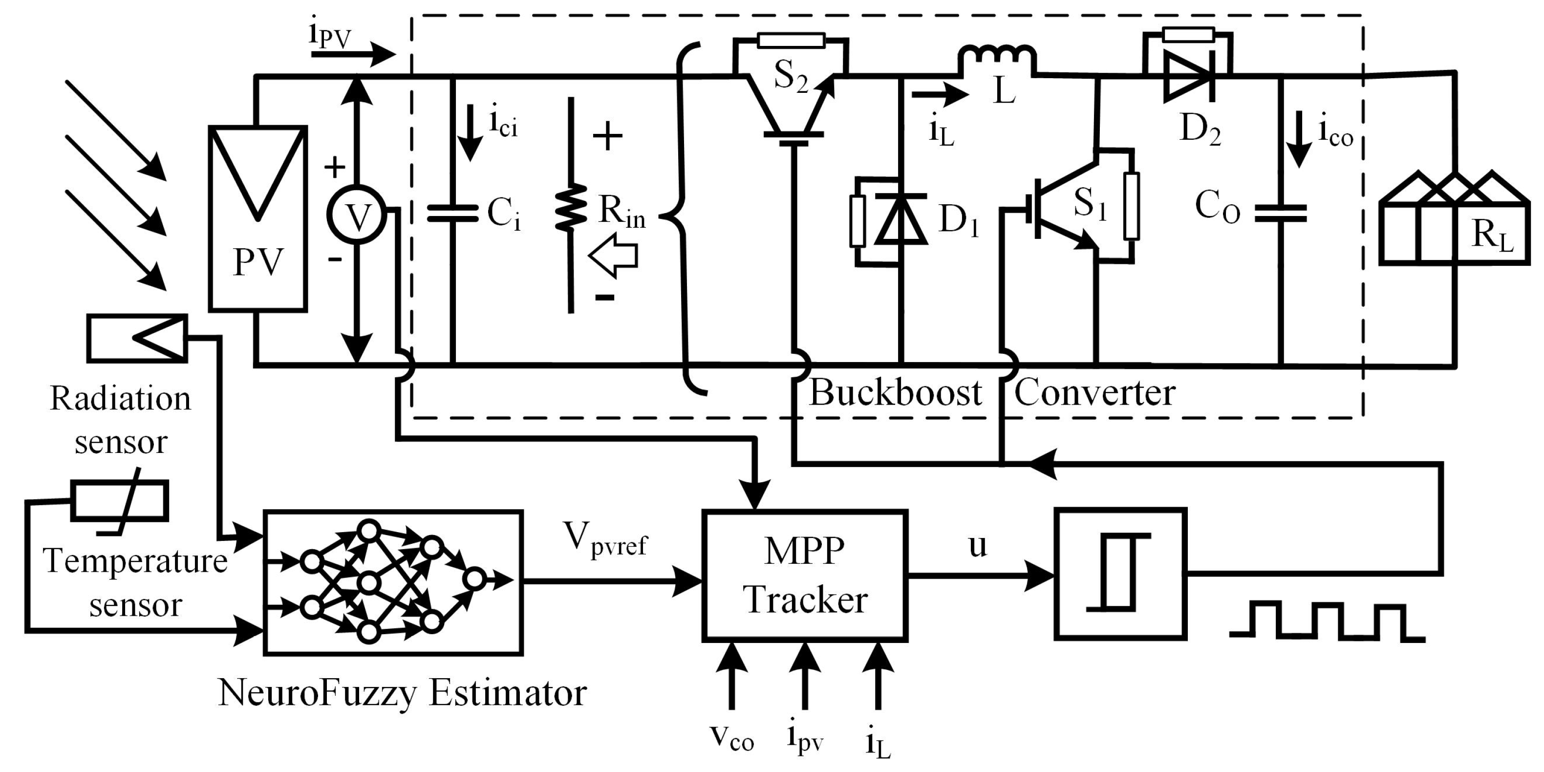
In [25,26], a nonlinear backstepping and integral backstepping controller is proposed to track maximum power point of PV array. However, a considerable steady-state error and overshoot was observed in backstepping and integral backstepping controllers, respectively during MPP tracking. Similarly, robustness of both the controllers have not been evaluated against certain faults or uncertainties occurring in the system. To mitigate these problems, a nonlinear robust integral backstepping-based MPPT control scheme is proposed in this research article, as shown in Figure 1. The proposed control scheme not only minimizes the steady-state errors and overshoots, but also outperforms the backstepping and integral backstepping controllers in terms of providing better efficiencies, better rise time, better peak time, better settling time with and without occurrence of certain faults or uncertainties in the system.

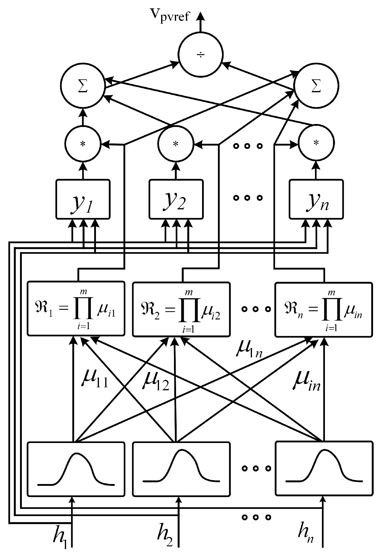
In this research article, a nonlinear robust integral backstepping controller is used for MPPT of PV array, using a non-inverting buck-boost converter. In Section 2, NeuroFuzzy network is presented. Mathematical modeling of the PV system is presented in Section 3. Section 4 presents state-space average modeling of the non-inverting DC-DC buck-boost converter. A nonlinear robust integral backstepping controller is presented in Section 6, whereas the analysis of global asymptotic stability is guaranteed through Lyapunov stability criteria in the corresponding section. The performance of the proposed controller for tracking MPP is analyzed under varying environmental conditions using MATLAB/Simulink. Simulation results are presented in Section 7 to show the effectiveness of the proposed controllers. Finally in Section 8, the conclusion is drawn.

2. Reference Voltage Generation by NeuroFuzzy Algorithm

NeuroFuzzy network used in this article is based on Takagi-Sugeno fuzzy inference system, which is shown in Figure 2, while a NeuroFuzzy-based nonlinear 3D-plane for PV array is depicted in Figure 3. The NeuroFuzzy network used has two inputs i.e, temperature and irradiance. The input layer is the fuzzification layer which has three Gaussian membership functions for each variable. The output layer has a linear equation for each rule. The NeuroFuzzy algorithm generates reference $V_{pvref}$ of the peak power voltage to extract maximum power from the PV array under varying environmental conditions.

3. Mathematical Modeling of PV System

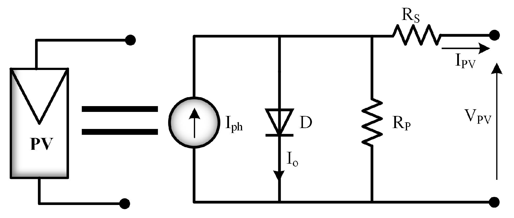
The PV cell have p-n junction similar to a diode, which produces the electric power by using photons. A PV cell consists of a series resistance, $R_s$, a shunt resistance, $R_p$, current source, $I_{ph}$ and a diode, D as shown in Figure 4. In order to extract the parameters of the equivalent electrical circuit, it is required to know the PV current-voltage or power-voltage curve in standard conditions of measurement (SCM). As $R_p$ has a high value and $R_s$ has a low one, so to simplify the study both can be neglected. The PV array electrical characteristics are often determined by the subsequent equations [27].

$$I_{pv}=N_p{I}_{ph}-N_p{I}_0\left[exp\frac{q{V}_{pv}}{N_{s}AKT}-1\right]$$

(1)

where $I_{pv}$ is the cell output current in $ampere$, A ideality factor of diode and $V_{pv}$ is the cell output voltage in V, q is electron charge in C, $N_s$ and $N_p$ are PV cells connected in series and parallel respectively, K is Boltzmann constant in $J/K$ and T is temperature in K.

Reverse saturation current, $I_0$ of the cell is given by:

$$I_0=I_{0r}{\left(\frac{T}{T_r}\right)}^{3}exp\left(\frac{q{E}_g}{KA}\left[\frac{1}{T_r}-\frac{1}{T}\right]\right)$$

(2)

where $E_g$ = 1.1 eV is energy gap or band gap of semiconductor and $T_r$ [K] is the cell reference temperature.

So, at $T_r$, the reverse saturation current, $I_{0r}$ is given by the following equation:

$$I_{0r}=\frac{I_{scr}}{exp\left(\frac{q{V}_{oc}}{N_{s}AKT}\right)-1}$$

(3)

where, $I_{scr}$ is the cell’s short circuit current at reference temperature, $T_r$ and radiation. $V_{oc}$ is the open circuit voltage.

The cell’s photocurrent, $I_{ph}$ depends on the irradiation, $E_e\left(\frac{W}{m^2}\right)$ and cell temperature, given by the following equation:

$$I_{ph}=\left[I_{scr}+K_i\left(T-T_r\right)\right]\frac{E_e}{1000}$$

(4)

where $K_i$ [A/K] is the temperature coefficient for short circuit current.

Power, $P_{pv}$ of the PV array can be calculated by the following equation:

$$P_{pv}=I_{pv}{V}_{pv}$$

(5)

$$P_{pv}=N_p{I}_{ph}{V}_{pv}-N_p{I}_0{V}_{pv}\left[exp\left(\frac{q{V}_{oc}}{N_{s}AKT}\right)-1\right]$$

(6)

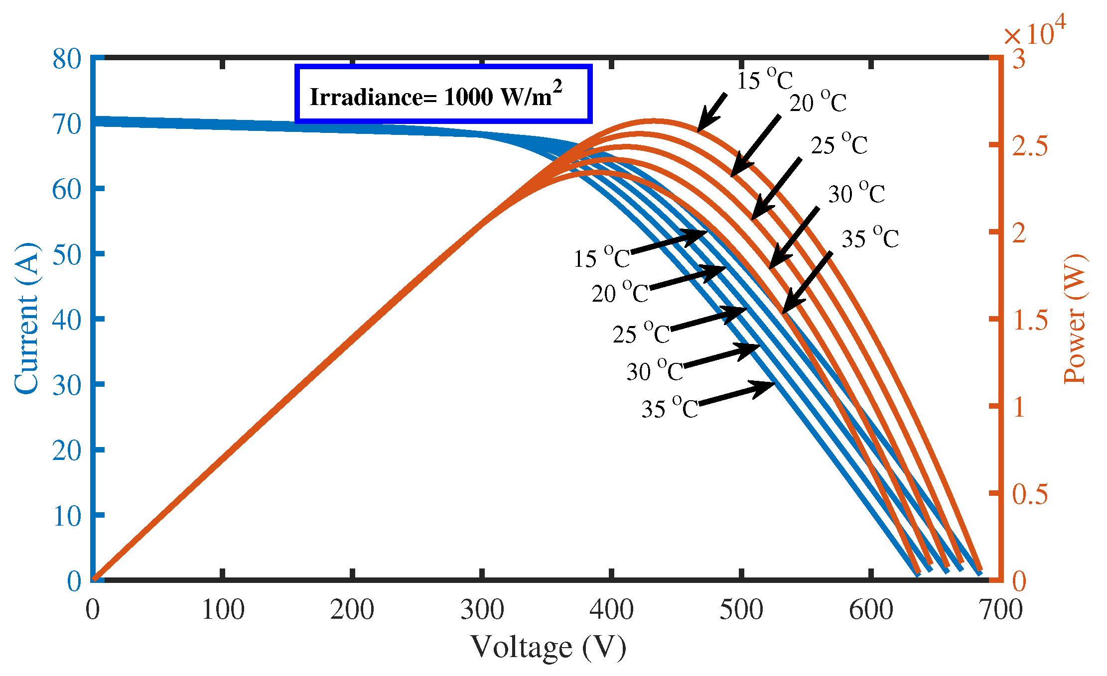
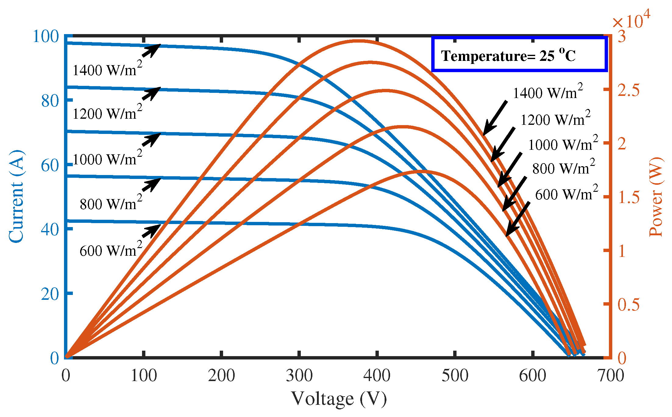
The PV array used in this paper consists of 4 strings which are connected in parallel. Every string consists of 4 modules connected in series. So, the total number of PV modules used in this paper are 16. One module has a power of 1555 W. So, the maximum power which can be delivered by this PV system is: 1555 × 16 = 24,880 W.

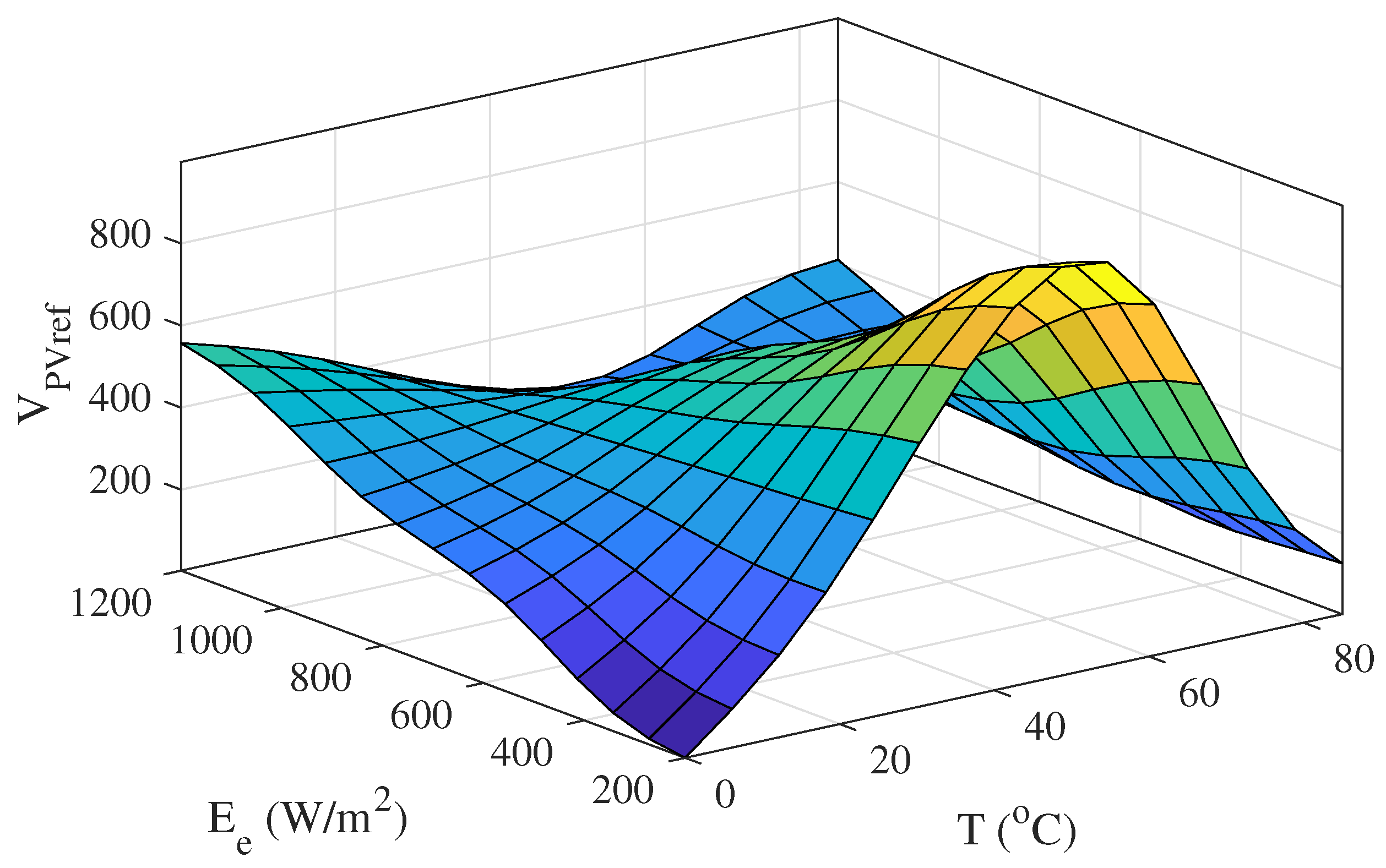
The PV array $\left(I_{pv}-V_{pv}\right)$ and $\left(P_{pv}-V_{pv}\right)$ characteristics for different values of temperature $\left(T\right)$ and solar irradiance $\left(E_e\right)$ is shown in Figure 5 and Figure 6, respectively.

4. Average State-Space Modeling of the Non-Inverting DC-DC Buck-Boost Converter

The non-inverting DC-DC buck-boost converter either steps up or steps down voltage from its input (PV array) to its output (load), in order to force the PV array to operate at the MPP. The converter is periodically controlled by its switching period, T where: $T=t_{on}+t_{off}$; $t_{on}$ is the ON time and $t_{off}$ is the OFF time, over this period. The duty ratio of the converter is defined as: $u=t_{on}/T$. The input capacitor, $C_i$, is used to limit ripples in the converter input voltage, while the output capacitor, $C_o$, is used to limit ripples in the output voltage. Throughout this paper, the converter is assumed to be operating in continuous conduction mode (CCM). The equivalent circuit of the non-inverting DC-DC buck-boost converter is shown in Figure 1, as a part of the complete model of the system [28].

There are two switching intervals. In the first switching interval, both the switches, $S_1$ and $S_2$ are ON while the diodes $D_1$ and $D_2$ are OFF. In the second switching interval, both the diodes $D_1$ and $D_2$ are ON while the switches, $S_1$ and $S_2$ are OFF.

The state-space equations for the first switching interval in vector-matrix form are as follows:

$$\left[\begin{array}{c}\frac{d{v}_{pv}}{dt}\\ \frac{d{i}_L}{dt}\\ \frac{d{v}_{c_0}}{dt}\end{array}\right]=\left[\begin{array}{ccc}0& -\frac{1}{C_i}& 0\\ \frac{1}{L}& 0& 0\\ 0& 0& -\frac{1}{R_L{C}_0}\end{array}\right]\left[\begin{array}{c}{v}_{pv}\\ i_L\\ v_{c_0}\end{array}\right]+\left[\begin{array}{c}\frac{i_{pv}}{C_0}\\ 0\\ 0\end{array}\right]$$

(7)

On the other hand, the state-space equations for the second switching interval in vector-matrix form are as follows:

$$\left[\begin{array}{c}\frac{d{v}_{pv}}{dt}\\ \frac{d{i}_L}{dt}\\ \frac{d{v}_{c_0}}{dt}\end{array}\right]=\left[\begin{array}{ccc}0& 0& 0\\ 0& 0& -\frac{1}{L}\\ 0& \frac{1}{C_0}& -\frac{1}{R_L{C}_0}\end{array}\right]\left[\begin{array}{c}{v}_{pv}\\ i_L\\ v_{c_0}\end{array}\right]+\left[\begin{array}{c}\frac{i_{pv}}{C_i}\\ 0\\ 0\end{array}\right]$$

(8)

Now, the average model for non-inverting DC-DC buck-boost converter with a resistive load in vector-matrix form based on inductor volt-second balance and capacitor charge-balance is as follows:

$$\left[\begin{array}{c}\frac{d{\overline{v}}_{pv}}{dt}\\ \frac{d{\overline{i}}_L}{dt}\\ \frac{d{\overline{v}}_{c_0}}{dt}\end{array}\right]=\left[\begin{array}{ccc}0& -\frac{\mu }{C_i}& 0\\ \frac{\mu }{L}& 0& \left(\frac{\mu }{L}-\frac{1}{L}\right)\\ 0& \left(\frac{1}{C_0}-\frac{\mu }{C_0}\right)& -\frac{1}{R_L{C}_0}\end{array}\right]\left[\begin{array}{c}{\overline{v}}_{pv}\\ {\overline{i}}_L\\ {\overline{v}}_{c_0}\end{array}\right]+\left[\begin{array}{c}\frac{i_{pv}}{C_i}\\ 0\\ 0\end{array}\right]$$

(9)

Assume $x_1$, $x_2$, $x_3$ and u as the average values of ${\overline{v}}_{pv}$, ${\overline{i}}_L$, ${\overline{v}}_{c_0}$ and $\overline{\mu }$, respectively. Under these assumptions, Equation (9) becomes as:

$$\left[\begin{array}{c}{\dot{x}}_1\\ {\dot{x}}_2\\ {\dot{x}}_3\end{array}\right]=\left[\begin{array}{ccc}0& -\frac{u}{C_i}& 0\\ \frac{u}{L}& 0& \left(\frac{u}{L}-\frac{1}{L}\right)\\ 0& \left(\frac{1}{C_0}-\frac{u}{C_0}\right)& -\frac{1}{R_L{C}_0}\end{array}\right]\left[\begin{array}{c}{x}_1\\ x_2\\ x_3\end{array}\right]+\left[\begin{array}{c}\frac{i_{pv}}{C_i}\\ 0\\ 0\end{array}\right]$$

(10)

The voltage transformation ratio of non-inverting DC-DC buck-boost converter is given as:

$$\frac{v_{c_0}}{v_{pv}}=\frac{u}{1-u}$$

(11)

The reflected input impedance based on ideal power transfer is given by [25]:

$$R_{opt}=R_{in}$$

(12)

where

$$R_{in}={\left(\frac{1-u}{u}\right)}^2{R}_L$$

and

$$R_{opt}=\frac{V_{MPP}^2}{P_{MPP}}$$

5. Robust Integral Backstepping Controller Design

In order to effectively track the reference voltage generated by a NeuroFuzzy algorithm and to extract maximum power from the PV array, a nonlinear robust integral backstepping MPPT controller is proposed. To proceed with the design, an error, $e_1$ is defined as the difference between the actual and the desired PV array output voltage, as:

$$e_1=x_1-x_{1ref}$$

(13)

where $x_{1ref}$ refers to $V_{pvref}$. The derivative of Equation (13) along the dynamics reported in Equation (10) becomes

$${\dot{e}}_1=\frac{i_{pv}}{C_i}-u\frac{x_2}{C_i}-{\dot{x}}_{1ref}$$

(14)

Since the objective is to steer the error signal $e_1$ to zero. Therefore, treating $x_2$ as a virtual control input which can be chosen according to Lyapunov stability theory. Thus, considering the time derivative of the Lyapunov candidate $V_1=\frac{1}{2}{e}_1^2$ along Equation (14), one comes up with

$${\dot{V}}_1=e_1{\dot{e}}_1=e_1\left(\frac{i_{pv}}{C_i}-u\frac{x_2}{C_i}-{\dot{x}}_{1ref}\right)$$

(15)

To introduce robustness into the backstepping strategy, $x_2$ becomes as:

$$x_2=\left(\frac{i_{pv}}{C_i}-{\dot{x}}_{1ref}+k_1{e}_1+k_{2}sign\left(e_1\right)\right)\frac{C_i}{u}$$

(16)

where $k_1$ and $k_2$ must be positive constants. With this choice of $x_2$, Equation (15) takes the form

$${\dot{V}}_1=-k_1{e}_1^2-k_2{e}_{1}sign\left(e_1\right)$$

(17)

Since the main objective is to provide a robust performance with almost zero steady-state error. Therefore, an integral action term $\lambda \varphi$, is added (i.e., integral backstepping strategy is adapted) to Equation (16). Consequently, one gets

$$x_{2ref}^{\prime }=\left(\frac{i_{pv}}{C_i}-{\dot{x}}_{1ref}+k_1{e}_1+k_{2}sign\left(e_1\right)\right)\frac{C_i}{u}+\lambda \varphi$$

(18)

where $\lambda$ is a constant, and $\varphi ={\int }_0^t{e}_{1}d\tau$. Now, treating $x_{2ref}^{\prime }$ as a new reference for the next step which will be tracked by the second state of the system. The tracking error is defined as follows:

$$e_2=x_2-x_{2ref}^{\prime }$$

(19)

and

$$x_2=e_2+x_{2ref}^{\prime }$$

(20)

Putting Equation (20) in Equation (15), one may get

$${\dot{V}}_1=e_1\left(\frac{i_{pv}}{C_i}-u\left(\frac{e_2+x_{2ref}^{\prime }}{C_i}\right)-{\dot{x}}_{1ref}\right)$$

(21)

$$=e_1\left(\frac{i_{pv}}{C_i}-u\frac{x_{2ref}^{\prime }}{C_i}-{\dot{x}}_{1ref}-u\frac{e_2}{C_i}\right)$$

Substituting Equation (18) in the above expression, one has

$${\dot{V}}_1=-k_1{e}_1^2-k_2{e}_{1}sign\left(e_1\right)-u\frac{e_2{e}_1}{C_i}$$

(22)

This inequality can also be written as:

$${\dot{V}}_1=-2k_1{V}_1-\sqrt{2}{k}_2\sqrt{V_1}-u\frac{e_2{e}_1}{C_i}$$

(23)

This differential inequality will be discussed at the end of this section. Now, differentiating Equation (20) with respect to time, it becomes

$${\dot{e}}_2={\dot{x}}_2-{\dot{x}}_{2ref}^{\prime }$$

(24)

where the time derivative of $x_{2ref}^{\prime }$ is calculated as follows:

$$\begin{array}{c}{\dot{x}}_{2ref}^{\prime }=\frac{1}{u^2}[\left(u\right)\left({\dot{i}}_{pv}-C_i{\ddot{x}}_{1ref}+k_1{C}_i{\dot{e}}_1\right)\hfill \\ -\left(i_{pv}-C_i{\dot{x}}_{1ref}+k_1{C}_i{e}_1+k_2{C}_{i}sign\left(e_1\right)\right)\left(\dot{u}\right)]\hfill \\ +\lambda e_1\hfill \end{array}$$

(25)

Carrying out some algebraic simplification, the expression of ${\dot{x}}_{2ref}^{\prime }$ becomes

$$\begin{array}{c}{\dot{x}}_{2ref}^{\prime }=\frac{1}{u}\left[{\dot{i}}_{pv}-C_i{\ddot{x}}_{1ref}-C_i{k}_1^2{e}_1-C_i{k}_1{k}_{2}sign\left(e_1\right)\right]\hfill \\ -k_1{e}_2-\frac{\dot{u}}{u}{x}_{2ref}+\lambda e_1\hfill \end{array}$$

(26)

Using it in Equation (24), one has

$$\begin{array}{cc}\hfill {\dot{e}}_2=& {\dot{x}}_2-[\left(\frac{1}{u}\right)\left({\dot{i}}_{pv}-C_i{\ddot{x}}_{1ref}-C_i{k}_1^2{e}_1-C_i{k}_1{k}_{2}sign\left(e_1\right)\right)\hfill \\ & -k_1{e}_2-\frac{\dot{u}}{u}{x}_{2ref}+\lambda e_1]\hfill \end{array}$$

(27)

A composite Lyapunov function, $V_c$, is defined to ensure convergence of the errors $e_1$ and $e_2$ to zero and the asymptotic stability of the system, as follows:

$$V_c=V_1+\frac{1}{2}{e}_2^2$$

(28)

The time derivative of $V_c$ along Equation (22) becomes

$${\dot{V}}_c=-k_1{e}_1^2-k_2{e}_{1}sign\left(e_1\right)+e_2\left({\dot{e}}_2-u\frac{e_1}{C_i}\right)$$

(29)

For $V_c$ to be negative definite, let

$${\dot{e}}_2-u\frac{e_1}{C_i}=-k_3{e}_2-k_{4}sign\left(e_2\right)$$

(30)

where $k_3$ and $k_4$ are positive constants. Using values of ${\dot{e}}_2$ from Equation (27) in Equation (30), it gives

$$\begin{array}{cc}\hfill -k_3{e}_2-k_{4}sign\left(e_2\right)=& -u\frac{e_1}{C_i}+{\dot{x}}_2-\left(\frac{1}{u}\right)\left({\dot{i}}_{pv}-C_i{\ddot{x}}_{1ref}-C_i{k}_1^2{e}_1-C_i{k}_1{k}_{2}sign\left(e_1\right)\right)\hfill \\ & +k_1{e}_2+\frac{\dot{u}}{u}{x}_{2ref}-\lambda e_1\hfill \end{array}$$

(31)

Now, making use of ${\dot{x}}_2$ from Equation (10) and solving for $\dot{u}$, one gets the final expression of the control law as follows:

$$\begin{array}{cc}\hfill \dot{u}=& \frac{1}{x_{2ref}}\left[e_2\left(-k_1-k_3\right)u-e_1\left(C_i{k}_1^2-\frac{u^2}{C_i}-u\lambda \right)+u\frac{x_3}{L}\right]+\hfill \\ & \frac{1}{x_{2ref}}\left[{\dot{i}}_{pv}-C_i{\ddot{x}}_{1ref}-u^2\left(\frac{x_1+x_3}{L}\right)-C_i{k}_1{k}_{2}sign\left(e_1\right)\right]\hfill \\ & +\frac{u}{x_{2ref}}\left[-k_{4}sign\left(e_2\right)\right]\hfill \end{array}$$

(32)

This choice of the control law guides Equation (29) to the forthcoming form

$${\dot{V}}_c=-k_1{e}_1^2-k_2{e}_{1}sign\left(e_1\right)-k_3{e}_2^2-k_4{e}_{2}sign\left(e_2\right)$$

(33)

This expression can also be written as follows:

$${\dot{V}}_c=-2{\overline{k}}_1{V}_c-\sqrt{2}{\overline{k}}_2{V}_c^{\frac{1}{2}}$$

(34)

where ${\overline{k}}_1=min(k_1,k_3)$ and ${\overline{k}}_2=min(k_2,k_4)$. The differential Equation (34) looks very similar to the fast terminal attractor [29]. This confirms that $V_c\to 0$ in finite time. In other words, $e_2=x_2-x_{2ref}^{\prime }\to 0$ in finite time which confirms high precisions in tracking as well as in regulation problems. As $e_2\to 0$ in finite time, the last term in the differential Equation (23) vanishes. Consequently, a terminal attractor in terms of $V_1$ is obtained which, once again, confirms the fast finite time convergence of $e_1$ to zero. Hence, the proposed control law (32) along with virtual control law (16) steers all the error dynamics to zero in finite time with high precision.

Now, the authors aim to present the stability of the zero dynamics. Since, a two step integral backstepping law is designed, so the dynamics

$${\dot{x}}_3=\left(\frac{1}{C_0}-\frac{u}{C_0}\right)x_2-\frac{1}{R_L{C}_0}{x}_3$$

(35)

are straight a way the internal dynamics of this PV system. According to the nonlinear theory [30], the zero dynamics can be obtained by substituting the applied control input u and the control driven states $x_1$ and $x_2$ equal to zero. Thus one has

$${\dot{x}}_3=-\frac{1}{R_L{C}_0}{x}_3$$

(36)

Since the typical parameters $R_L$ and $C_0$ are positive, therefore, Equation (36) has poles in the left half plane at $-\frac{1}{R_L{C}_0}$. This validates that the zero dynamics are exponentially stable and confirms the minimum phase nature of the under study PV system. Now, in the forthcoming section the simulation results will demonstrate the effectiveness of the proposed law in sound details.

6. Simulation Results and Discussion

Matlab/Simulink (SimPowerSystems toolbox) is used to simulate the PV array model, the average non-inverting DC-DC buck-boost converter model and the proposed MPPT technique. The information about PV array, non-inverting DC-DC buck-boost converter and controllers used in this study is given in

Table 1. Parameters of the PV system.

Type	Name of Parameters	Symbols	Magnitude
PV Module	Maximum power	$P_{max}$	1555 W
	Number of Cells per module	$N_s$	72
	Voltage at maximum power	$V_{mp}$	102.6 V
	Open circuit voltage	$V_{oc}$	165.8 V
	Short circuit current	$I_{sc}$	17.56 A
	Current at maximum power	$I_{mp}$	151.16 A
Converter	Input Capacitor	$C_i$	$1\times {10}^{-3}$ F
	Inductor	L	$20\times {10}^{-3}$ H
	Output capacitor	$C_0$	$48\times {10}^{-6}$ F
	Load resistance	$R_L$	50 $\Omega$
	IGBT switching frequency	$f_s$	5000 Hz
RIB Controller	Constant	$k_1$	60
	Constant	$k_2$	9000
	Constant	$k_3$	2000
	Constant	$k_4$	10
	Constant	$\lambda$	29
PID Controller	Gain	$k_p$	1.74
	Gain	$k_d$	1
	Gain	$k_i$	2.33

.

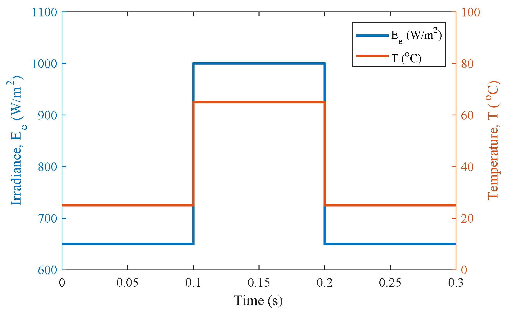
The proposed MPPT technique is evaluated from three different aspects i.e., $\left(1\right)$ robustness to climatic changes, $\left(2\right)$ faults and $\left(3\right)$ uncertainties. The irradiance and temperature profiles are depicted in Figure 7.

6.1. Robustness to Climatic Changes

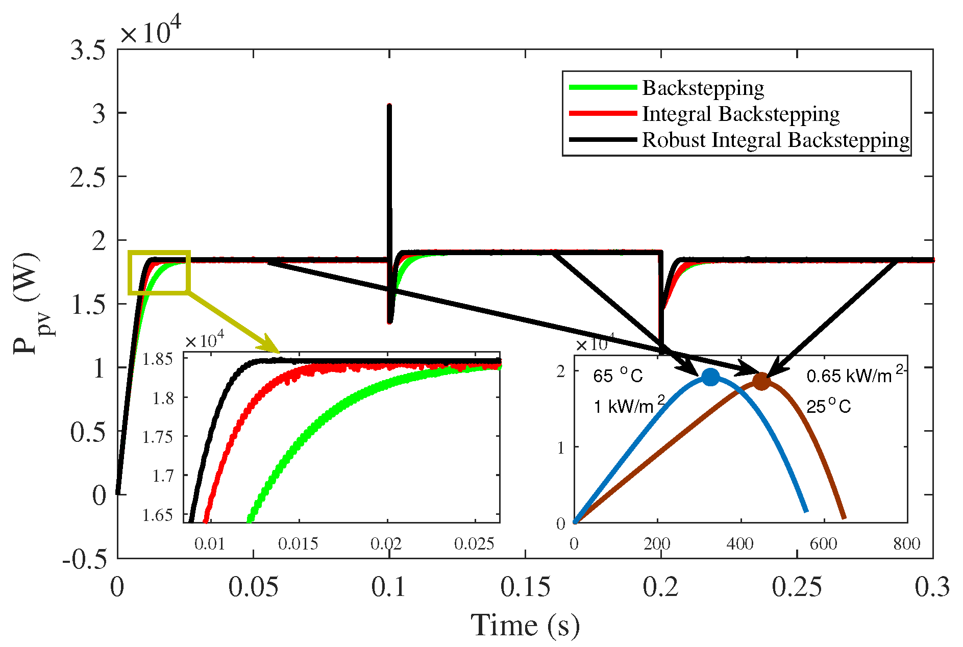
In this case, temperature, irradiance as well as load is varied to validate the robustness of the proposed MPPT technique. In the first time interval $t=[0,0.1]$ (s), temperature is maintained at 25 ${}^{\circ }$C, irradiance at 650 W/m${}^2$ and load at 30 $\Omega$, and the maximum PV power is $18.4$ kW. In the second time interval $t=[0.1,0.2]$ (s), temperature is changed to 65 ${}^{\circ }$C, irradiance to 1000 W/m${}^2$ and load to 40 $\Omega$, and maximum PV power is $19.02$ kW. Finally, in the time interval $t=[0.2,0.3]$ (s), the temperature is settled back to 25 ${}^{\circ }$C, irradiance to 650 W/m${}^2$ and load to 50 $\Omega$, and maximum PV power is $18.4$ kW.

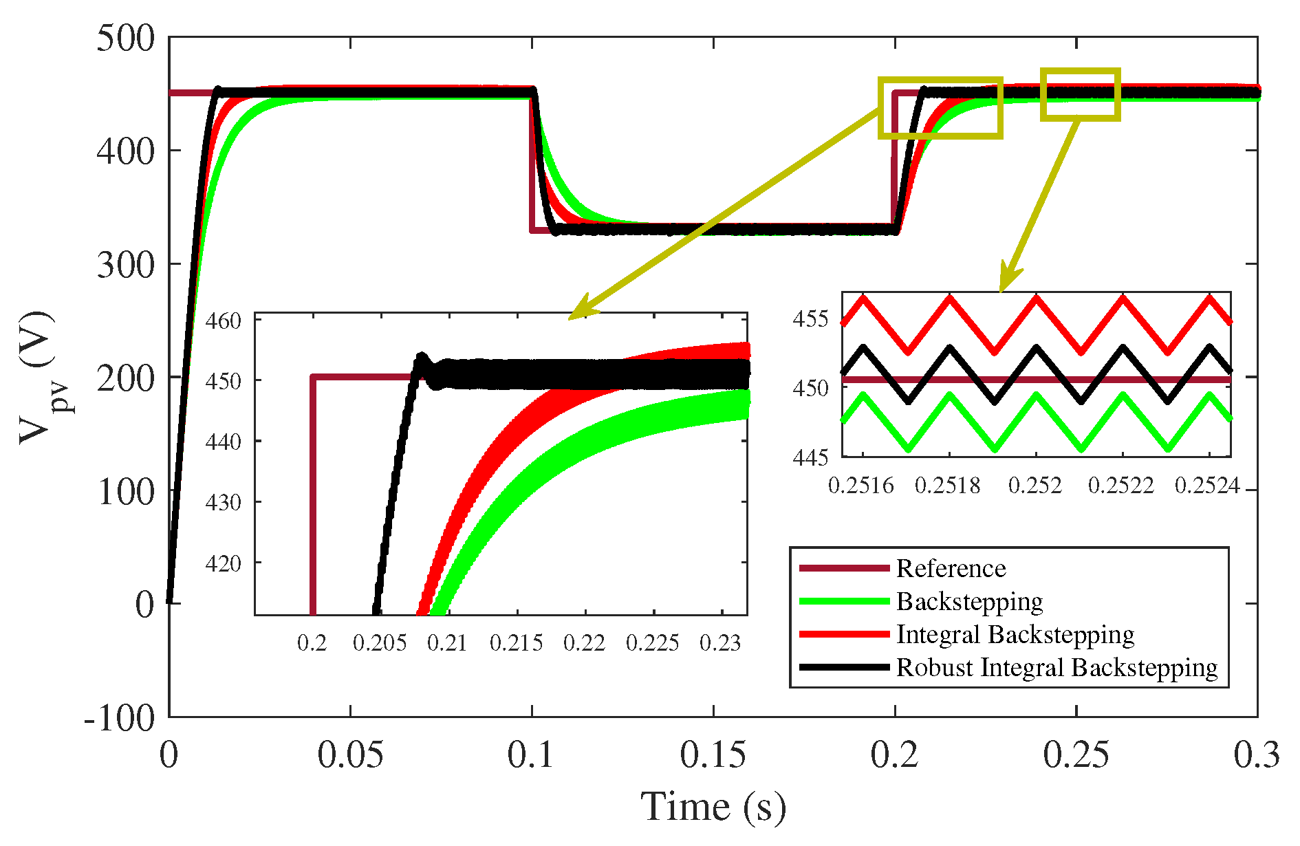
Reference, $V_{ref}$ of the peak power voltage generated by NeuroFuzzy network, is successfully tracked by all the three controllers. However, it can be observed that the proposed controller reaches steady-state at all levels at 0.01 s, again which is faster compared to the other MPPT techniques, as shown in Figure 8.

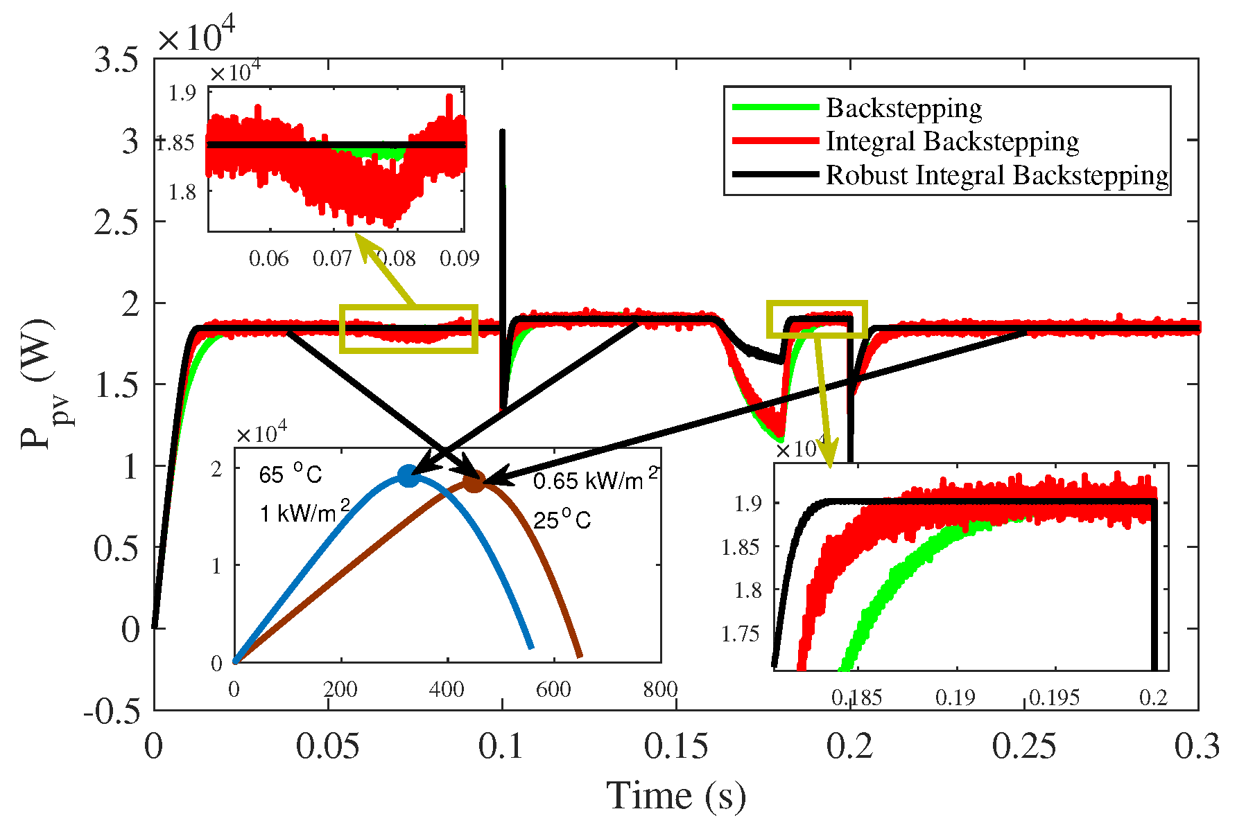
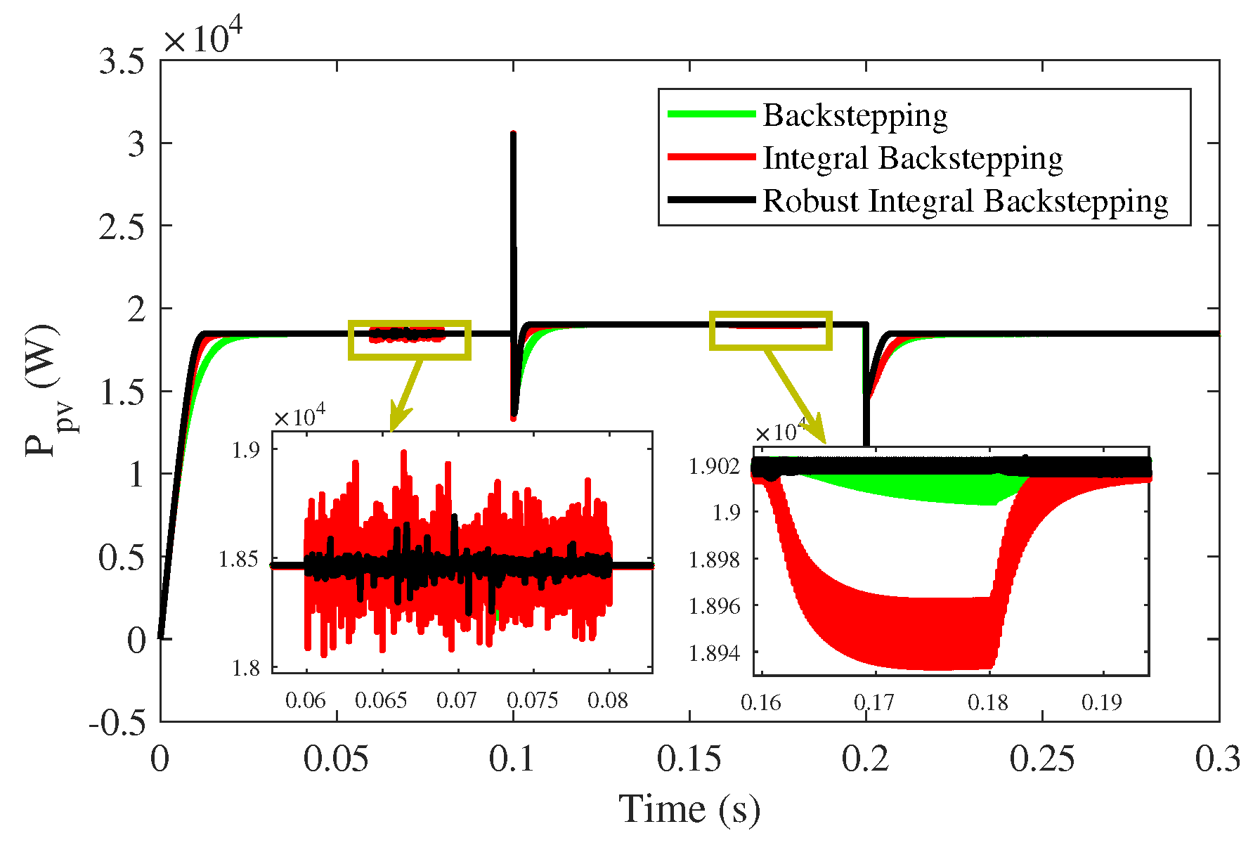
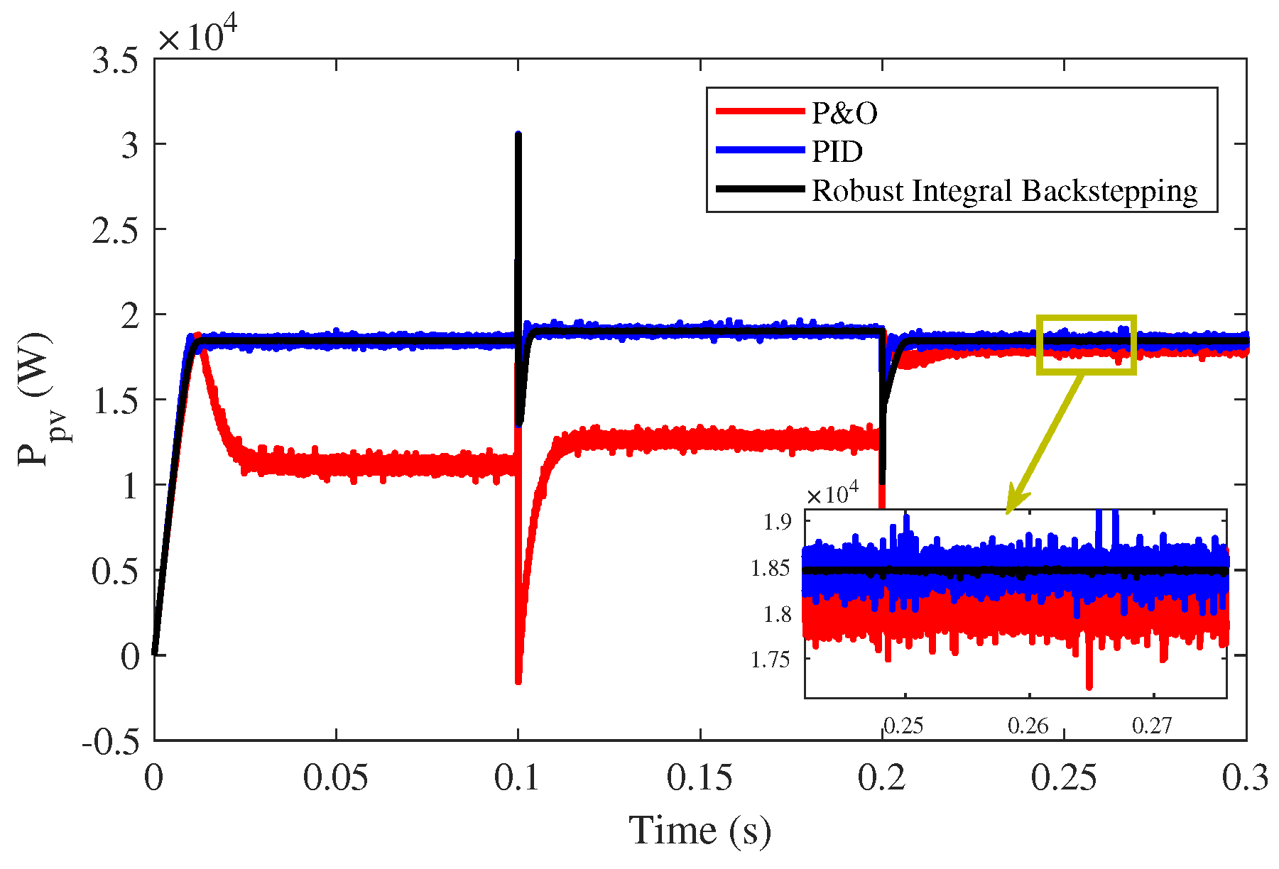
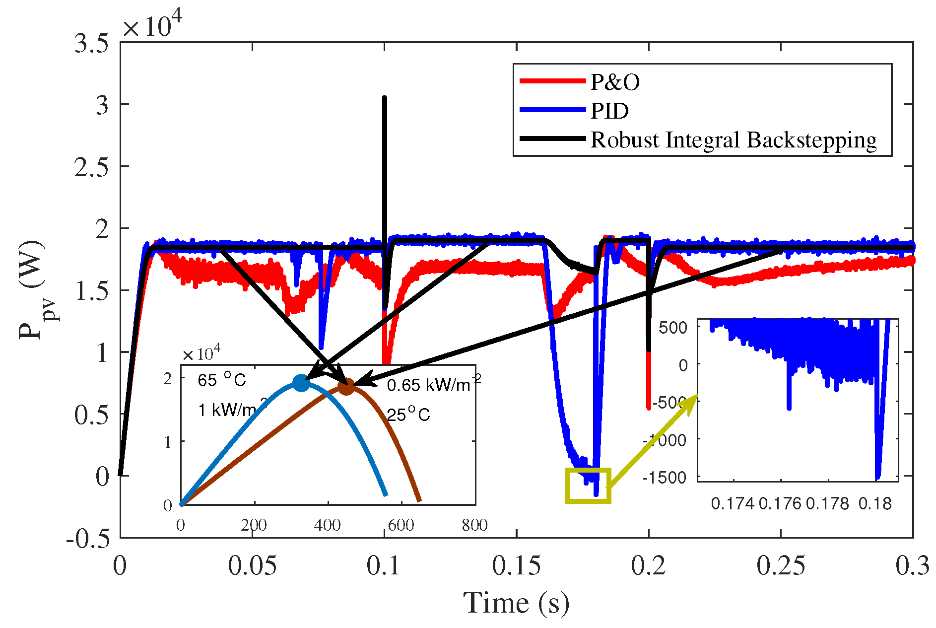
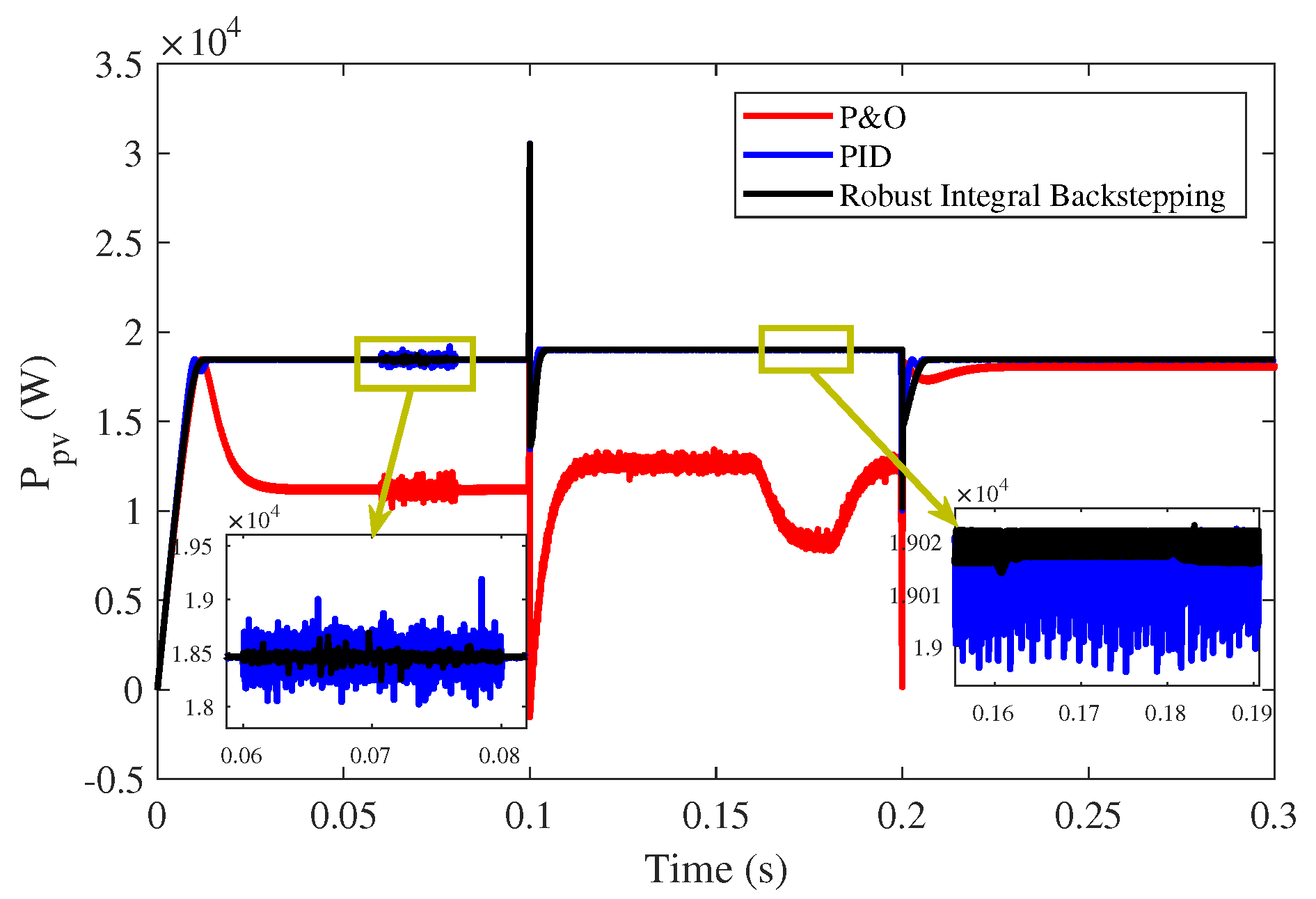
PV array output power along with MPP curves is shown in Figure 9. It can be observed that MPP is successfully achieved by the proposed controller within 0.01 s, with almost negligible ripples, compared to other MPPT techniques.

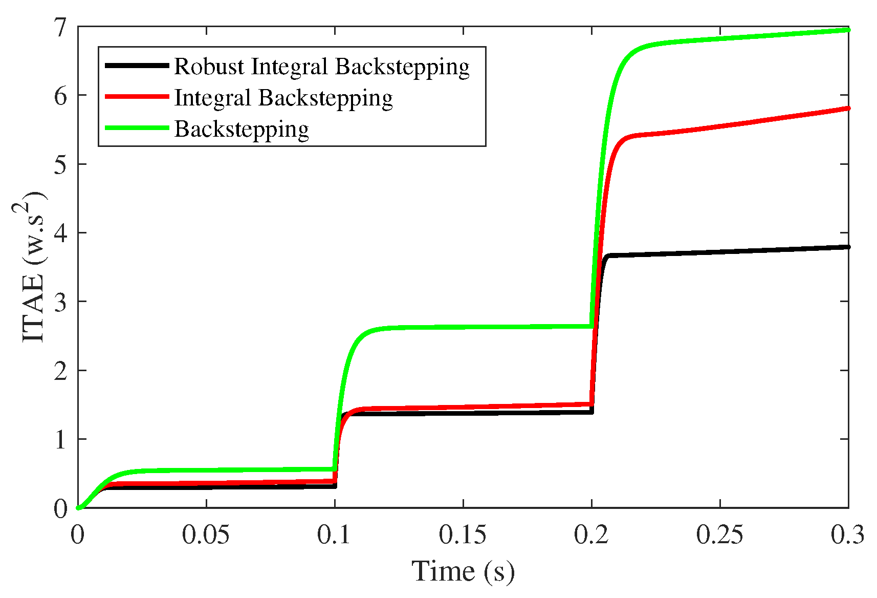
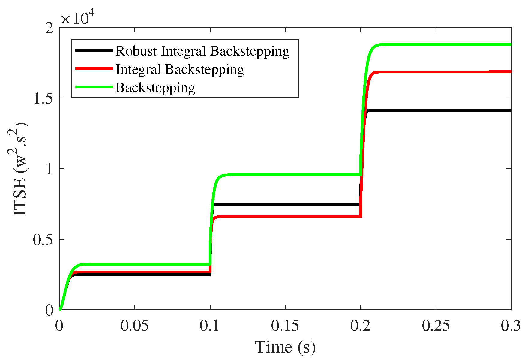
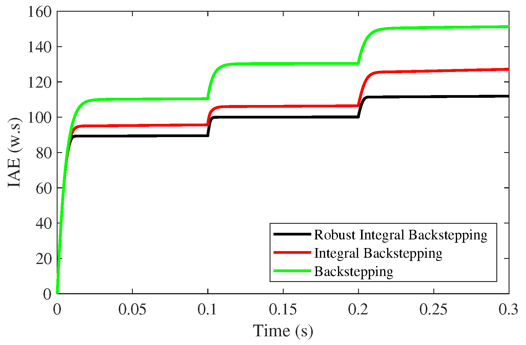
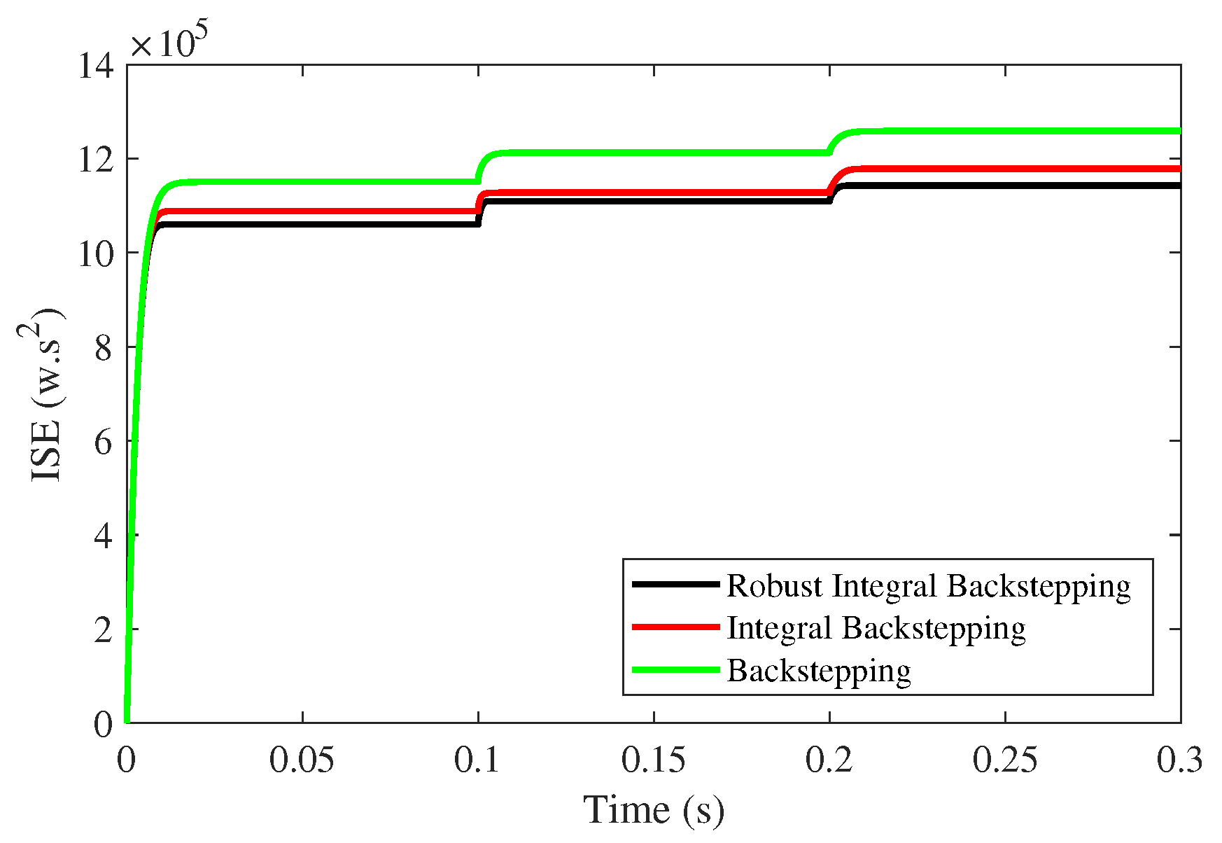
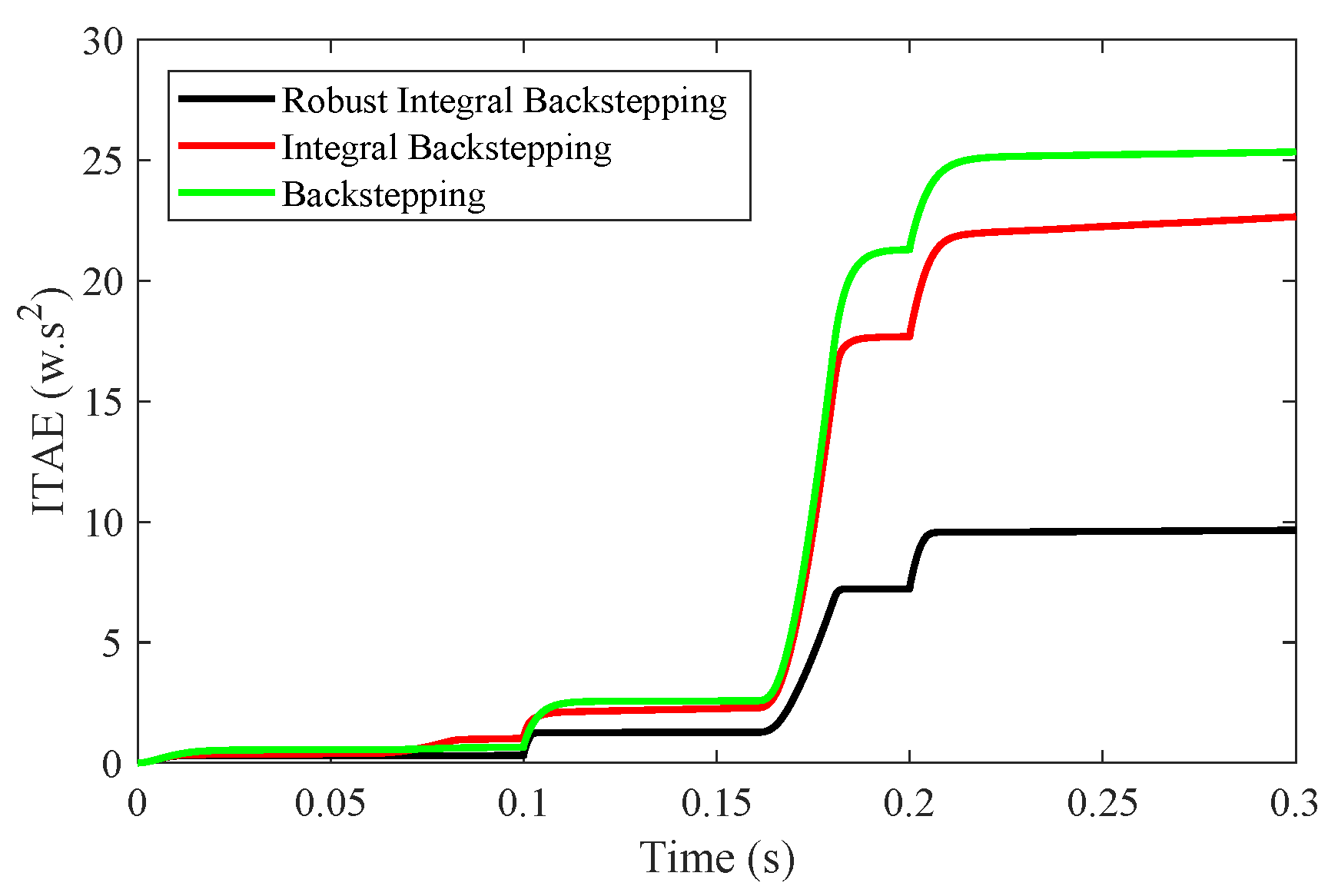
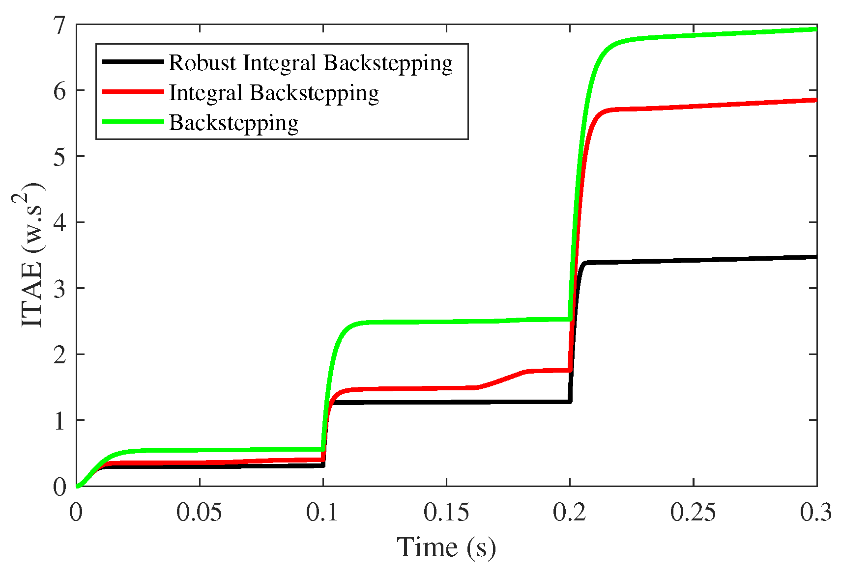
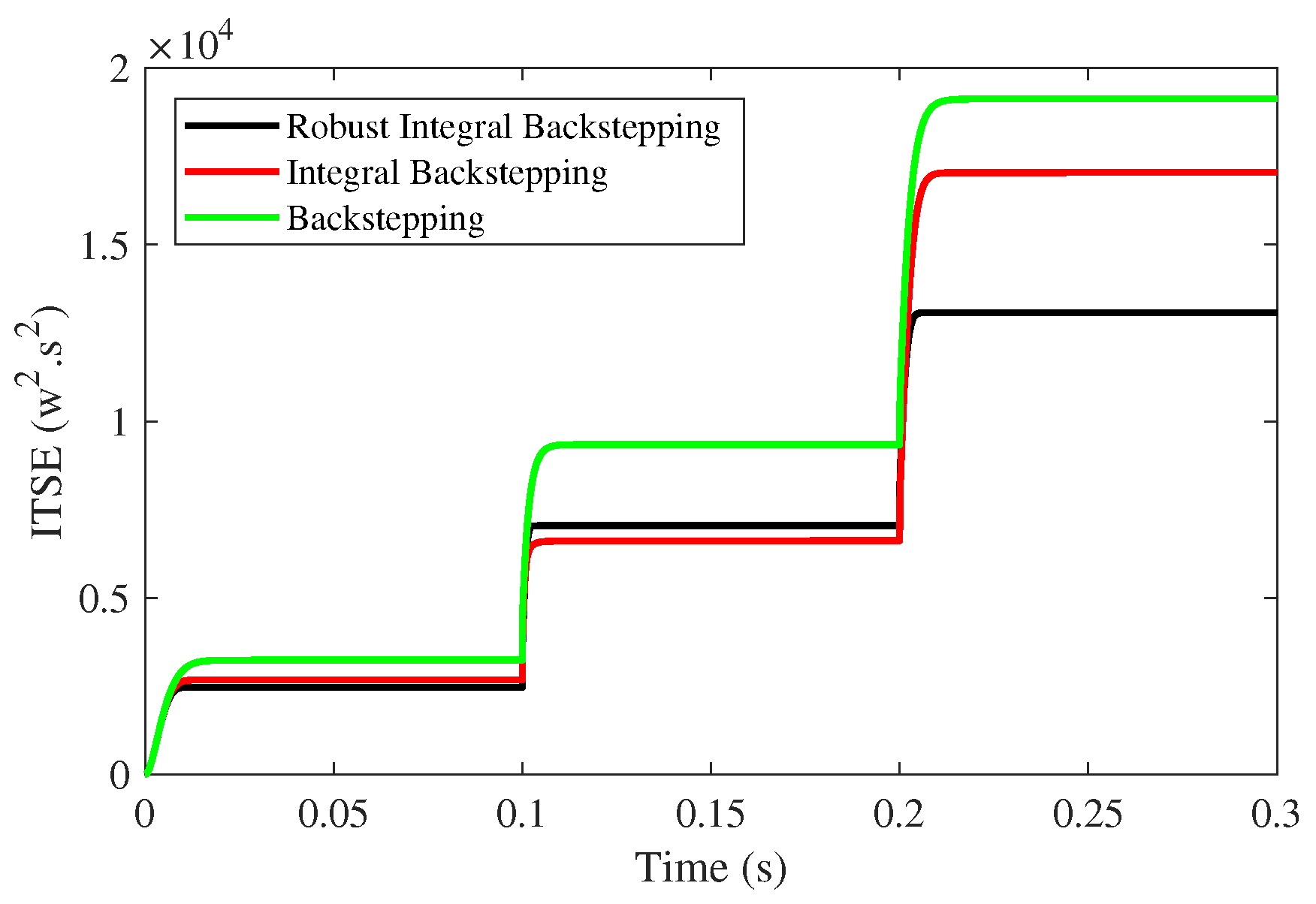
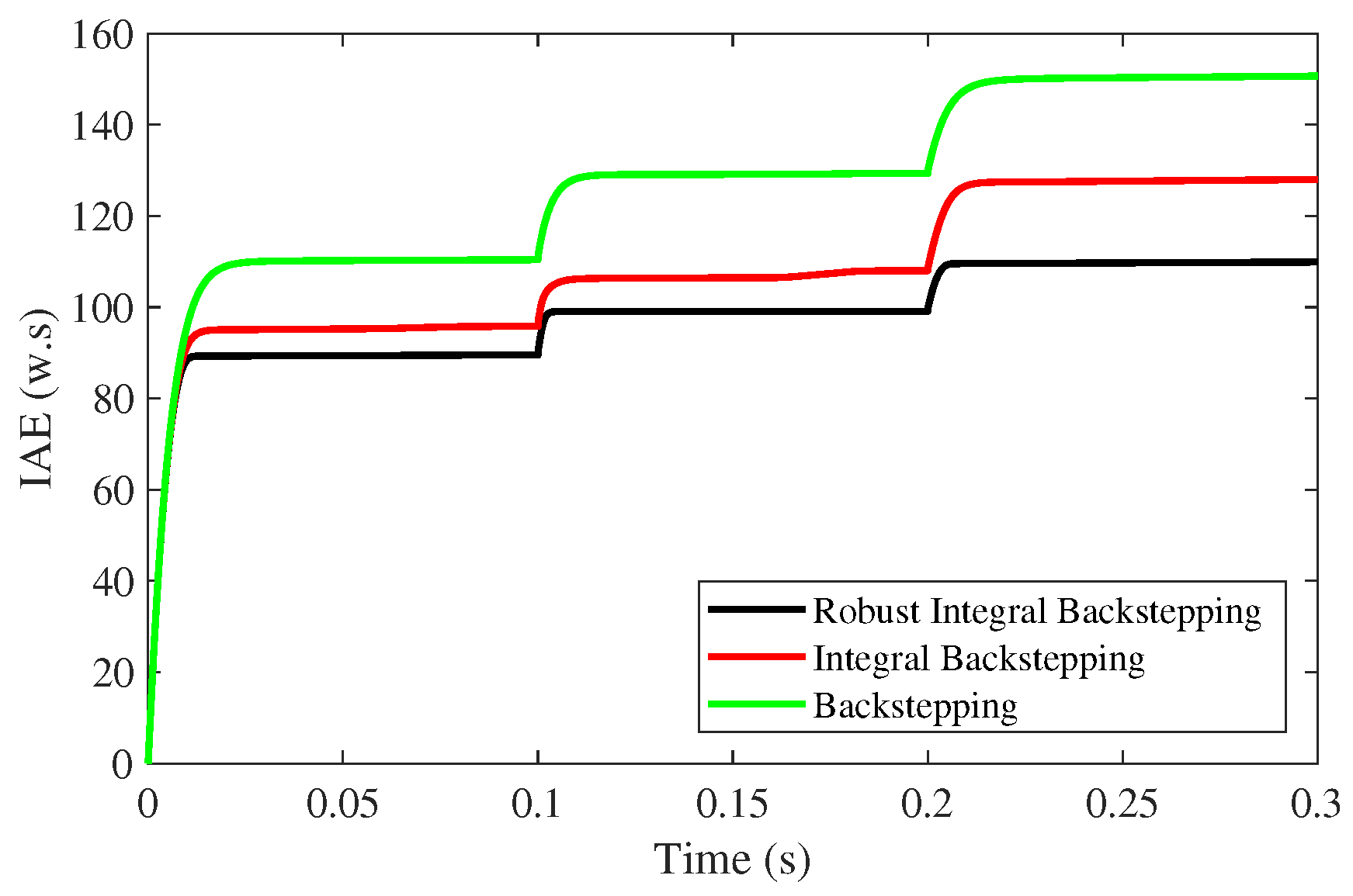
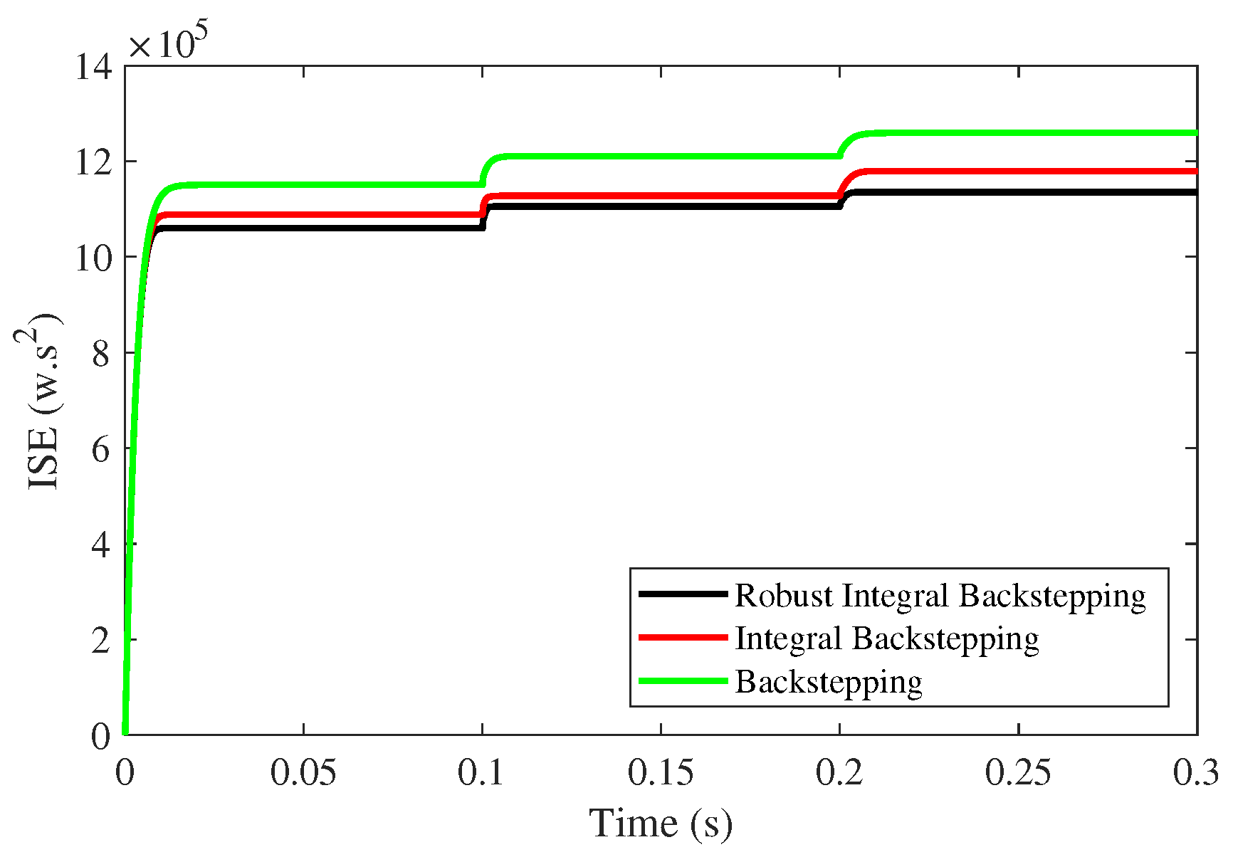
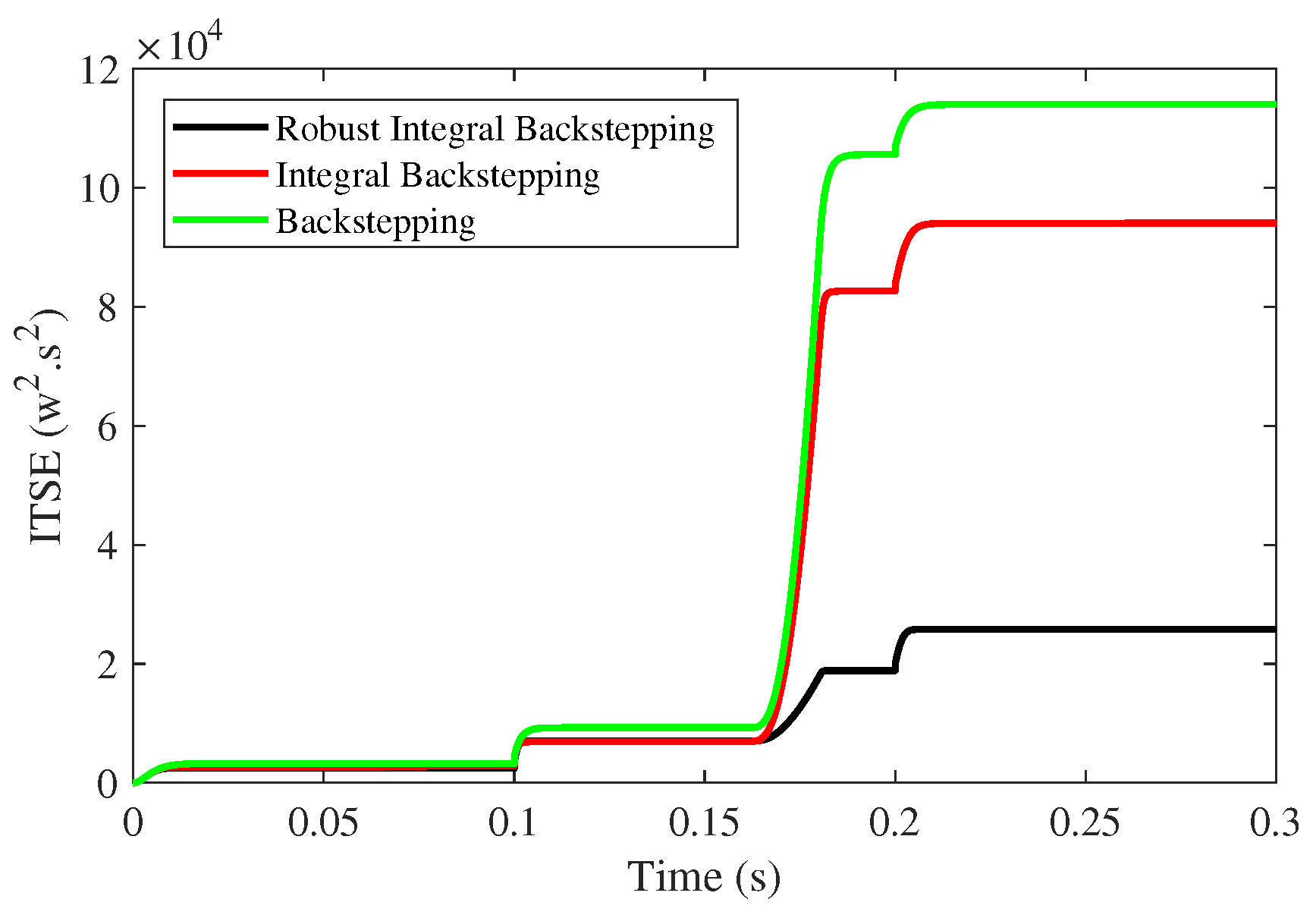
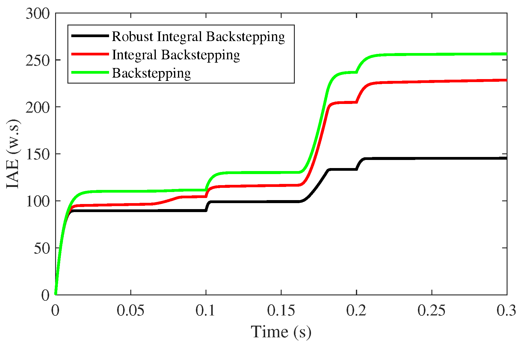
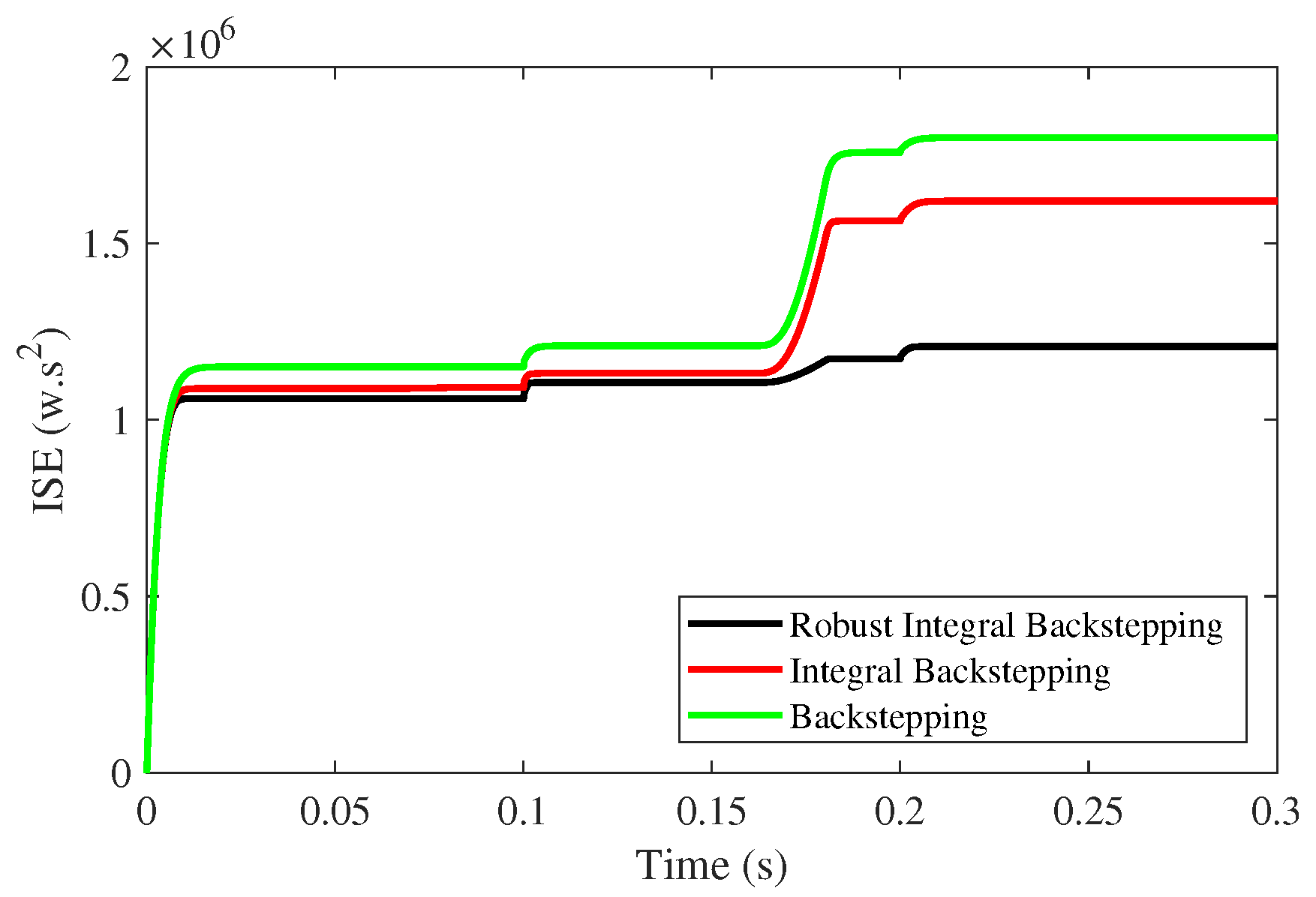
Figure 10, Figure 11, Figure 12 and Figure 13 depicts performance indexes IAE (Integral Absolute Error), ITAE (Integral Time Absolute Error), ISE (Integral Square Error) and ITSE (Integral Time Square Error) of the PV system. The superiority of the proposed technique has been verified based on these performance indexes.

Similarly, maximum power is transmitted to load by the proposed robust integral backstepping controller with efficiency of $98.04\%$, which is maximum compared to other MPPT techniques.

In this manner, the validation of the robustness of the proposed robust integral backstepping controller under varying temperature, irradiance and load is guaranteed.

6.2. Robustness to Faults under Climatic Changes

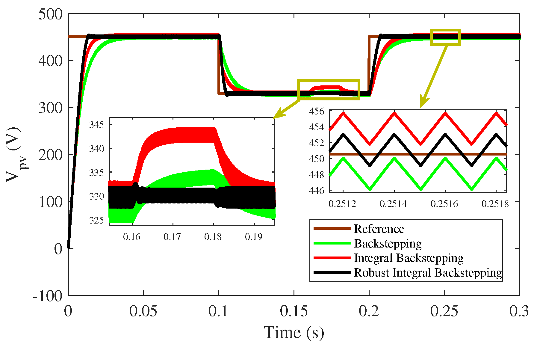
In this case, multiple faults are introduced under varying irradiance, temperature and load condition. In the time interval $t=[0.06,0.08]$ (s), a fault, $x_{3f}=30usin\left(t\right)/C_i$, is added to output voltage capacitor $x_3$, as $\Delta x_3=x_3+x_{3f}$. A second fault $x_{2f}=0.5usin\left(t\right)/C_i$, is added to inductor current $x_2$, in the time interval $t=[0.16,0.18]$ (s), as $\Delta x_2=x_2+x_{2f}$.

The PV output voltage deviates from the $V_{ref}$, due to occurrence of faults in the system, as shown in Figure 14. However, the proposed controller deviates from 329 V to 415 V, which is minimum deviation from $V_{ref}$ compared to integral backstepping from 329 V to 470 V and backstepping from 329 V to 476 V, in the time interval $t=[0.16,0.18]$ (s). Also, in the time interval $t=[0.06,0.08]$ (s), a fault deviates the backstepping controller from $V_{ref}=450$ V to 412 V and integral backstepping controller from 450 V to 412 V, while the proposed controller shows robustness against fault. It can be observed that the proposed controller reaches steady-state faster than other controllers. Besides, a maximum steady-state error is observed in backstepping controller after faults occurrence.

Figure 15 depicts the PV array output power. It is clear that proposed controller performs the best, and reaches steady-state quickly in 0.002 s after faults, with almost negligible ripples.

The performance indexes of PV system (IAE, ITAE, ISE and ITSE), as shown in Figure 16, Figure 17, Figure 18 and Figure 19 validate the effectiveness of the proposed control scheme. Also, maximum power is transmitted to load by the proposed robust integral backstepping controller with efficiency of more than $95\%$, outperforming the other MPPT techniques.

6.3. Robustness to Uncertainties under Climatic Changes

In this case, multiple uncertainties are introduced under varying irradiance, temperature and load condition. In the time interval $t=[0.06,0.08]$ (s), uncertainty of $\Delta L$ = 200 mH, is added to inductor L, as $L_t=L+\Delta L$. A second uncertainty of $\Delta C$ = 0.48 $\mathsf{\mu }$F, is added to output capacitor $C_0$, in the time interval $t=[0.16,0.18]$ (s), as $C_t=C_0+\Delta C$.

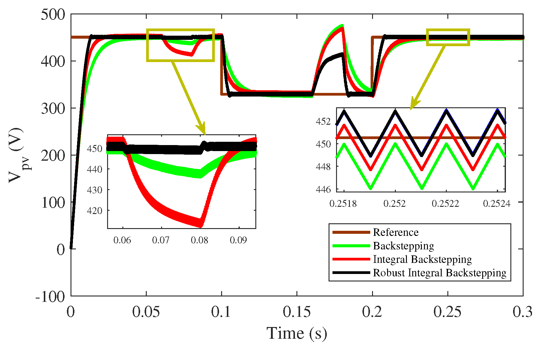
From Figure 20, it can be observed that backstepping controller deviates about 6 V and integral backstepping controller 15 V from the $V_{ref}$, while there is no deviation in the proposed controller. Besides, a maximum steady-state error is observed in backstepping and integral backstepping.

In Figure 21, it is clear that the proposed controller has negligible ripples and no deviation from MPP.

Similarly, in Figure 22, Figure 23, Figure 24 and Figure 25 the performance indexes of PV system (IAE, ITAE, ISE and ITSE) are depicted. These results validate that the proposed technique performs better than the other MPPT techniques.

Also, maximum power is transmitted to load by the proposed robust integral backstepping controller with efficiency of $98.07\%$, which is maximum compared to the other MPPT techniques.

7. Comparison with Conventional Techniques

The performance of the proposed robust integral backstepping controller is further validated by comparing its performance with conventional P&O and PID MPPT controllers.

7.1. Robustness to Climatic Changes

First conventional techniques (P&O and PID) are compared with the proposed robust integral backstepping technique under the same test (robustness to climatic changes).

The proposed MPPT technique outperforms the conventional PID and P&O techniques. Under varying temperatures, irradiance and load, the PV array output power is shown in Figure 26. It can be seen that the proposed MPPT technique is not only robust, but also the ripples are negligible. Moreover, one can observe that the proposed technique presents a very fast system reaction against meteorological conditions. The PID controller performs better than the P&O technique but results in oscillations around MPP.

Also the proposed robust integral backstepping controller transmitted maximum power to load with efficiency of $98.7\%$, which is greater than the efficiencies of PID and P&O MPPT techniques.

7.2. Robustness to Faults under Climatic Changes

Again the same test (robustness to faults under climatic changes) was performed to compare the performance of conventional PID and P&O with the proposed robust integral backstepping controller.

Figure 27 shows the PV output power under faults condition. It can be seen that due to the occurrence of faults in the system, PID controller deviates from MPP to negative power, while the P&O technique does not track MPP at all. However the proposed controller shows robustness against faults with almost negligible ripples.

Moreover, the proposed robust integral backstepping controller transmits maximum power to the load with efficiency of $98.6\%$.

7.3. Robustness to Uncertainties under Climatic Changes

In this case, the performance of the PID and P&O are compared with the proposed robust integral backstepping under the same test (robustness to uncertainties under climatic changes).

It is clear from Figure 28 that the proposed technique has much smaller ripples in the output power due to uncertainties as compared to those produced in PID and P&O controllers.

Also, maximum power is transmitted to load by the proposed robust integral backstepping with efficiency of $98.6\%$, outperforming the conventional PID and P&O MPPT techniques.

It can be noted that the desirable performance of the proposed robust integral backstepping in various conditions has been maintained and tracking operations have been carried out as well.

8. Conclusions

In this article, a nonlinear robust integral backstepping MPPT technique is proposed. A NeuroFuzzy network is used to generate the reference voltage for MPPT. Asymptotic stability of the system is guaranteed using Lyapunov stability criteria. The robustness of the proposed technique is investigated by simulation under climatic changes, uncertainties and faults. Results clearly showed that the proposed robust integral backstepping controller tracks the MPP quickly and accurately compared to PID, P&O, backstepping and integral backstepping. The simulation results validate the high performance of the proposed robust integral backstepping controller in terms of steady-state error, tracking accuracy, overshoot, rise time, settling time and efficiency. The simulation results verify the superiority of the proposed robust integral backstepping controller.