2.1. Proposed Method
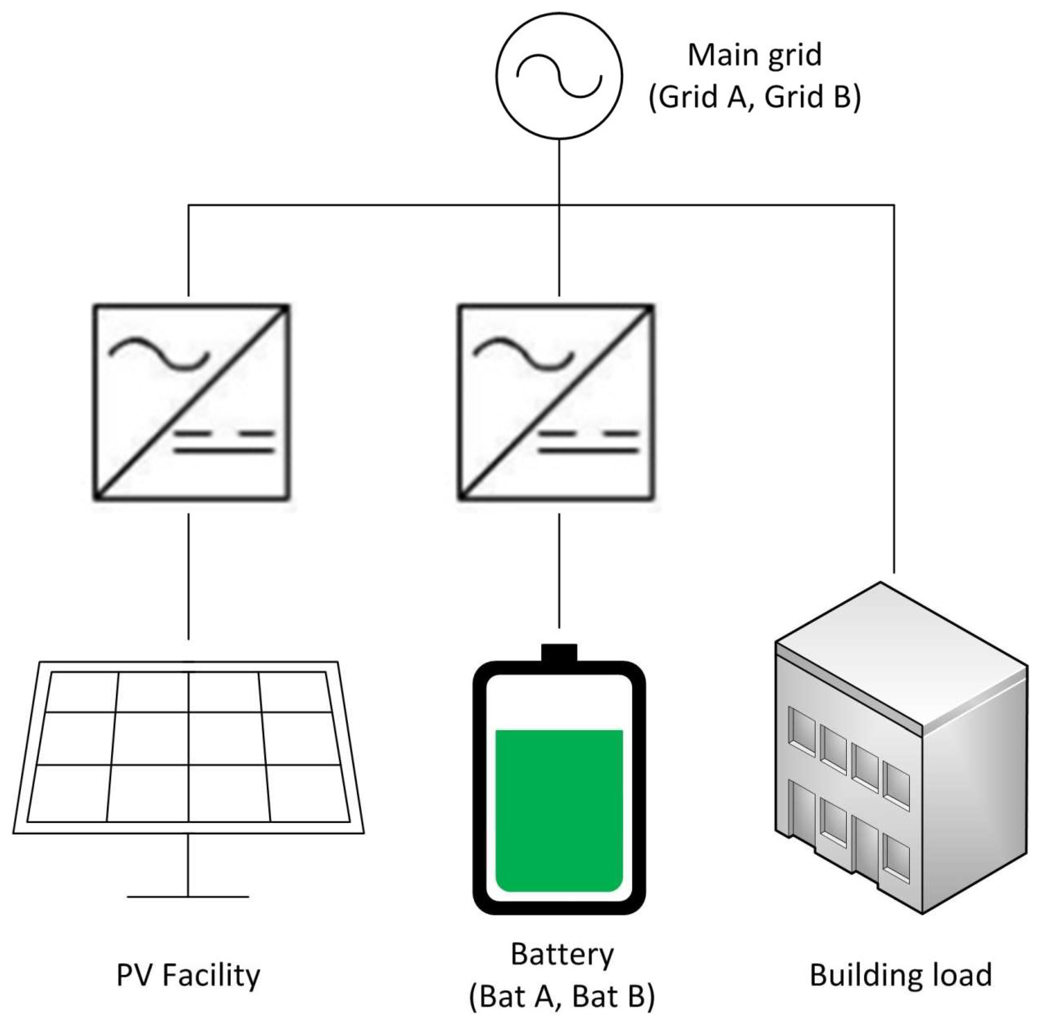
The proposed method is designed to optimally use an energy storage system on a microgrid with a load and generation system connected to the distribution grid. For the rest of this document, a battery and a PV facility will be assumed to play the energy storage and generation systems, as those were employed during the tests.
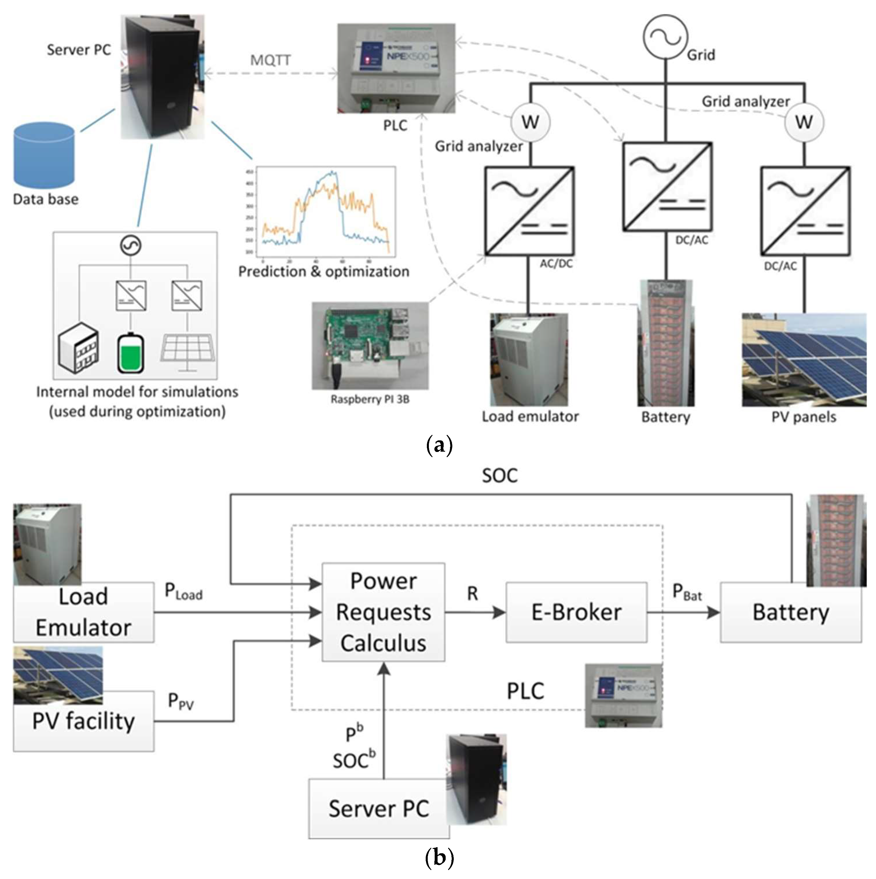
Figure 1 shows the model of the microgrid.
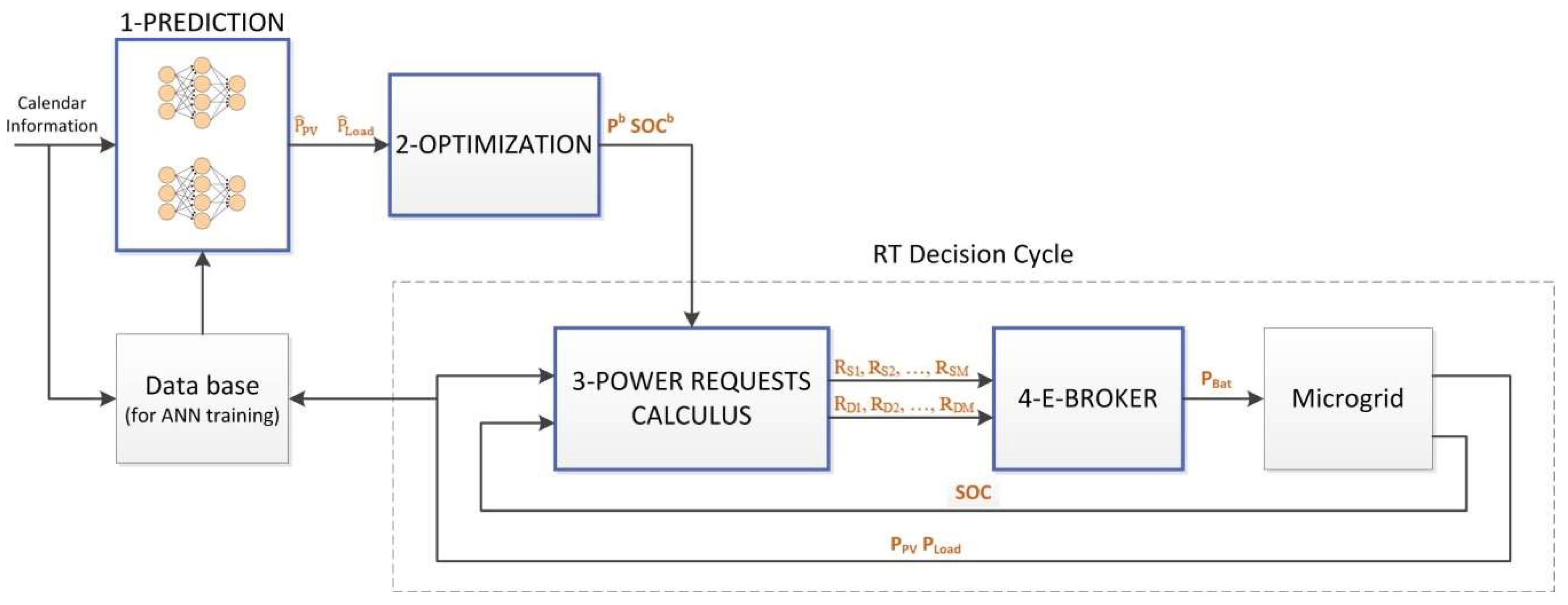
The method comprises four key operations: a prediction, an optimization, several power requests definitions, and an auction. The prediction and the optimization are applied once a day, while the power requests and the auction are executed continuously as a real time (RT) decision cycle.
The power requests (R), which are made on behalf of the devices of the microgrid, represent how much power each device is capable provide as a supplier (RS) or absorb as a demander (RD). For example, a power request is associated with the PV facility and indicates how much power it can provide. Similarly, a power request is associated with the load indicating how much power it will consume. Power requests are made for all devices, including the main grid. The auction algorithm, or E-Broker, then calculates how much power must be transferred between the different devices according to these power requests and a priority system. The power requests corresponding to the battery and main grid are split, as if they were respectively modeled as two batteries (Bat A and Bat B) and two main grids (Grid A and Grid B). The E-Broker treats these power requests with different priorities, so the whole system will behave differently depending on how these power request divisions are made. These power requests divisions (between Grid A and B, and between Bat A and B) depend on two variables: Pb and SOCb.
The values of Pb and SOCb are obtained through the aforementioned optimization process. At the beginning of each day, a heuristic optimization function chooses the best evolution of these variables along the day to reduce the expected electricity bill as much as possible. To do so, the optimization process considers the initial state of the battery and the electricity prices. Additionally, since the load consumption and the PV generation cannot be controlled (except for generation curtailment), the optimization process considers a prediction for the power consumed or generated by these devices. This prediction is made just before the optimization process.
Figure 2 shows the inputs and outputs of each operation. These operations are further described below in its own subsection. The whole method has been programed in Python.
2.1.1. Prediction
As previously stated, the optimization process needs some prediction of the uncontrolled devices power: the load and the PV facility. The more accurate the prediction is, the more reliable the optimization will be. Nevertheless, the strategy employed to obtain this prediction is not a fundamental part of the general method. The procedure described here was used to obtain the results of
Section 3; other prediction methods, like the future work mentioned in
Section 4, would work as well.
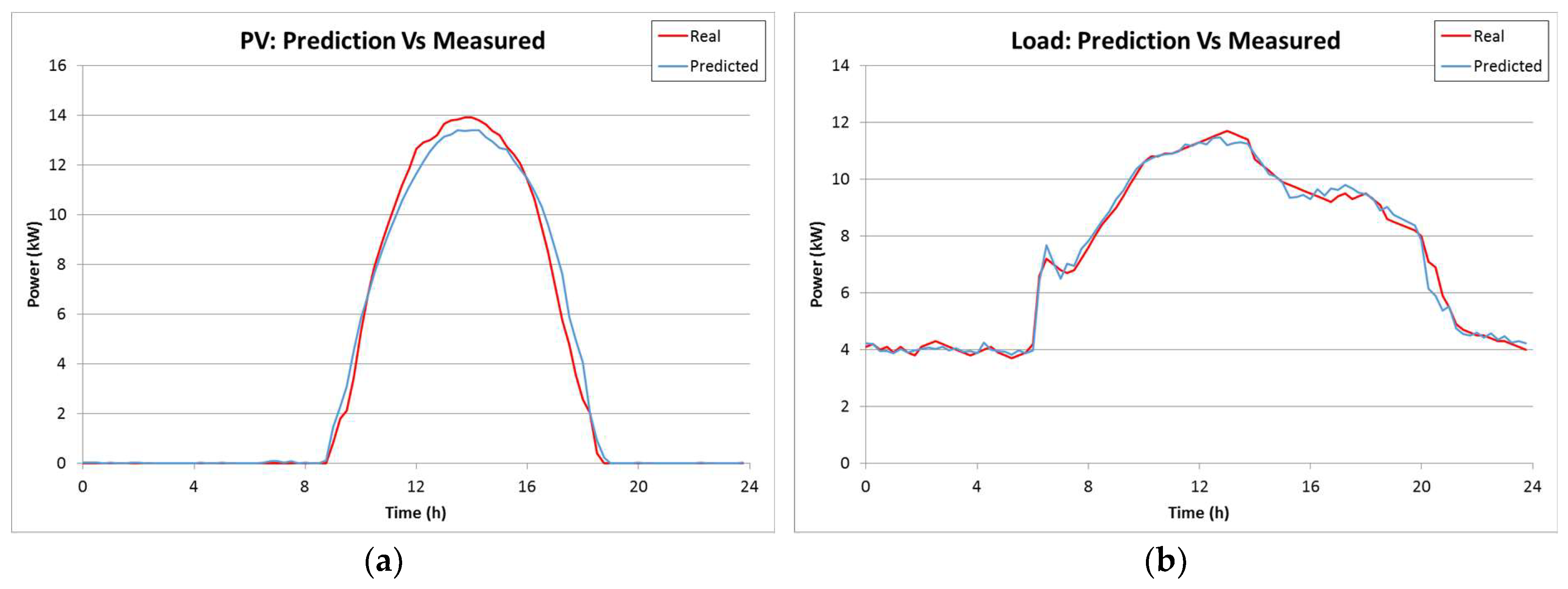
Predictions of loads and generation are obtained at the beginning of each day using artificial neural networks (ANNs). These predictions occur at midnight and consider only calendar information: the month, the day of the week, and the type of day (working day or holiday). For the tests, the load corresponded to a laboratory building in the University of Seville. Since the usage of the building follows a schedule, the calendar information is enough to obtain good predictions. The PV facility is harder to predict as it depends on the weather. However, calendar information is good enough for average and cloudless days. In the future, more weather-related inputs will be included to cover the possibility of cloudy days.
The ANNs used for the tests have been programmed in Python using the Keras package for Deep Learning, which runs on top of Theano (see [
28] for more information about the Keras package). The activation function of the ANNs uses the rectifier activation function or Rectified Linear Unit (ReLU). The mean square error is minimized in the compilation. The “adam” efficient gradient descent algorithm is also used for its high efficiency. The number of iterations run for the training process (epochs) is 200. The number of evaluated instances before updating the weights (batch size) is 2.
Two ANNs are used for the predictions: one for the PV () facility and another for the load (). The ANNs are structured in three layers of 70, 50, and 96 neurons; with 3 inputs for calendar information and 96 outputs for the predicted quarter-hourly power values. These output power values are assumed to be the average power produced or consumed by the corresponding device during a 15-min window. All ANNs have been trained with 1-year historical data, using 70% of the data for training and the remaining 30% for evaluation.
2.1.2. Optimization
After the prediction, an optimization process is run to find the best suited evolution for Pb and SOCb according to the prediction. These values will later serve as boundaries to determine the behavior of the grid and the battery regarding the power auction.
The selected algorithm for this optimization is the PSO, which is typical and efficient for this type of problem according to [
15]. If the priorities of the E-Broker auction, which only consider relative order, needed to be optimized, then the genetic algorithm (GA) would be suitable. This is so because the GA works better with discrete variables. However, the proposed priorities are already optimal for this microgrid. Since PSO works better than GA for continuous variables, PSO is preferred.
The PSO method is imported from library pyswarm for Python. The swarm size is specified to be 2000 particles. The stop conditions are also specified: the maximum number of iterations is 200, the minimum step of the particles is 0.0001 and the minimum change of the objective function is 0.0001€/month. This way, once iterations have no real impact on the yearly electricity cost, the method stops. The default values are used for the remaining parameters, which define the movement of the particles.
Aside from the upper and lower limits of Pb and SOCb, no constraints need to be imposed. This is so because the power requests and the auction algorithm always command the battery to exchange a feasible amount of power with another device capable to do so. The absence of constraints ensures a connected and convex space of candidate solutions, which simplifies the movement of the particles in the PSO.
The optimization variables are the necessary parameters to parametrize Pb and SOCb. Pb is a boundary for the grid power that triggers a different behavior of the grid regarding the power requests. The grid power requests will have a higher priority as long as the grid power is below Pb. Tests indicate that the best evolution for Pb is to remain constant, so it can be defined with only one optimization variable xp. Pb is chosen to be proportional to the contracted power Pcont and to the optimization variable xp, which is bounded between 0 and 1. Although this is not expected, Pb is allowed to be greater than the contracted power.
Similar to Pb, SOCb is a boundary for the battery state of charge (SOC) that triggers different power requests. Several piecewise polynomial interpolations have been tested to parametrize the best behavior of SOCb with the PSO selecting both the time and the SOCb value for each point. Best results have been obtained with a lineal interpolation between 13 points for each day. The first is at midnight and its value corresponds to the actual SOC of the battery at the time of the optimization. The last point is 24 h later. Both coordinates of the remaining points, as well as the value of SOCb for the last point, are optimization variables for the PSO algorithm. Variables that define the time coordinate of these points are bounded between 0 and 1, which correspond to the beginning and the end of the day respectively. Variables that define the SOCb coordinates are bounded between 0.1 and 0.95, which correspond to 10% and 95% of the battery allowed SOC range.
The objective function is the total grid electricity cost for a month with 30 equal days according to Spanish tariff 3.0A. This tariff considers the time of use (TOU) for energy and power by dividing the day into three periods with different prices. On each period, the energy cost depends on the total amount of energy provided by the grid during each period while the power cost depends on the highest power peak P
Peak of each period. Details of these costs can be consulted on [
29]. At the moment of writing this paper, the Spanish legislation does not allow consumers to sell electricity, so this situation is not considered. Nevertheless, it is possible to consider this case by adding power requests on behalf of the grid as a demander.
To evaluate the objective function, the PSO simulates the actions of the RT decision cycle (the Power requests calculus and the E-Broker auction algorithm) according to the values of Pb and SOCb. Thus, each evaluation of the objective function requires simulating a day divided into 96 equal intervals of 15 min. Please note that the sample time of the actual RT decision cycle is 5 s. The 15-min sample time is just a simplification to be able to run so many simulations. On all these simulations, the load and the PV facility are assumed to consume or generate the previously predicted average power for each interval.
Each simulation obtains the total energy cost C
ETotal as
where C
E k and P
Grid k are the energy cost and the power provided by the grid during interval k. The total power cost C
PTotal is calculated as
where C
P k and P
Peak k are the power cost and the maximum peak registered for period k, and function f(P
Peak k) is defined according to the Spanish legislation.
P
cont is the contracted power, which can be changed once a year if the user so desires, but for the optimization it is considered to be a known constant. The value of the objective function F
Obj is calculated by adding the total energy cost of 30 equal days and the total power cost for the month:
2.1.3. Power Requests Calculus
Power requests are calculated on real time according to the measures and optimization values. Afterwards, they are sent to the E-Broker auction algorithm, where they function similar to power bids. Several power requests may be associated with the same device.
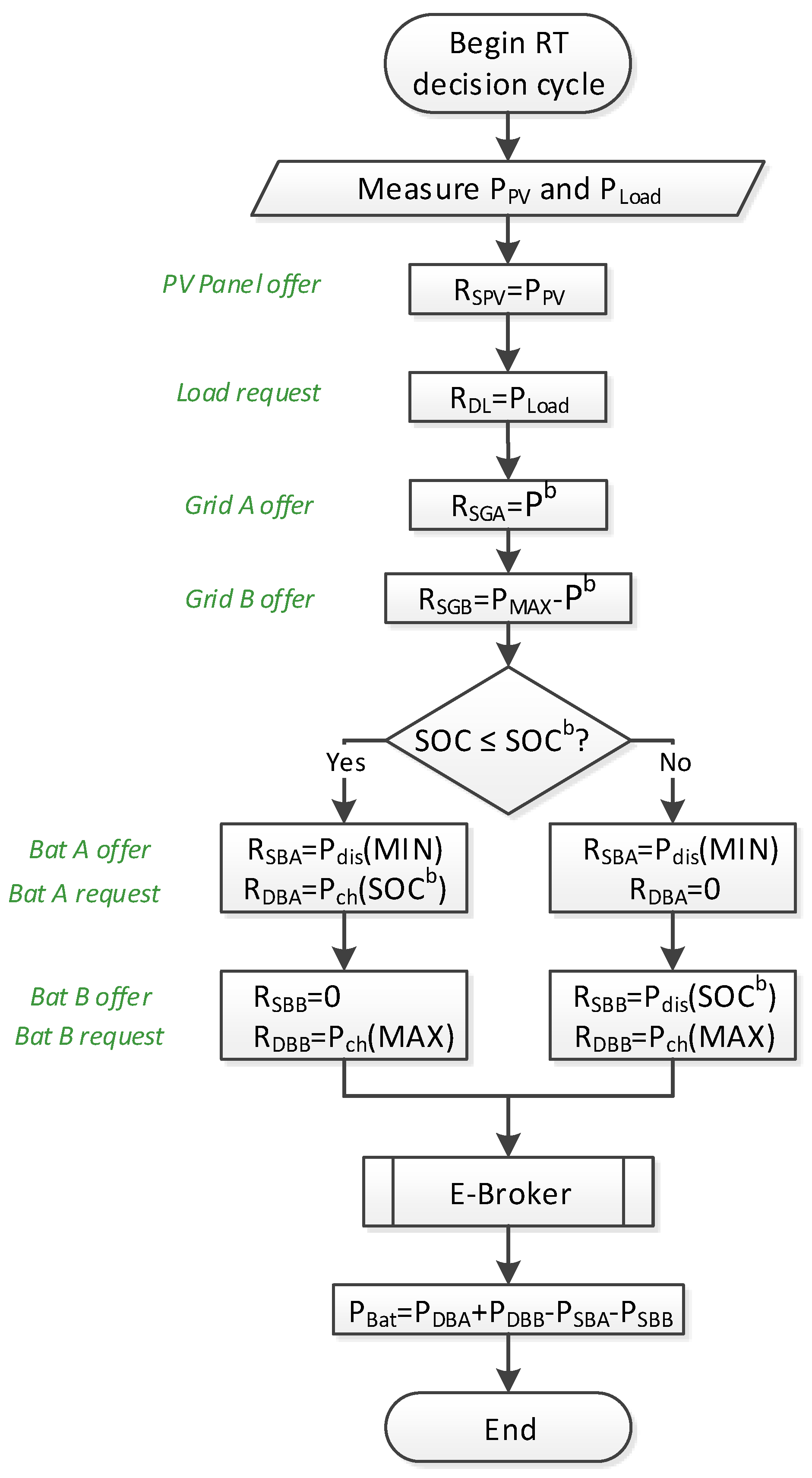
Figure 3 summarizes how the values of power requests are calculated for each device.
The actual power generated by the PV facility PPV and the power consumed by the load PLoad are measured. A power request is made on behalf of each one (RSPV and RDL) to provide or receive the same power they are respectively generating or consuming. These two devices are not actually requesting permission to produce or consume such power; they will do it anyway as they are not controlled. Thus, to ensure the E-Broker auction algorithm always serves these requests, they will be given the highest priority.
The power grid is associated to two power requests: RSGA and RSGB. This can be understood as dividing the grid into two different suppliers (Grid A and Grid B) that, together, can provide up to the grid maximum power PMAX. The value of RSGA is Pb, the optimal power limit of the grid. The rest of the power the grid can provide is assigned to RSGB. RSGA will later have a higher priority than RSGB, so an attempt will be made to limit the grid power to Pb. Nevertheless, thanks to RSGB, it is possible to go beyond this limit, if absolutely necessary.
The battery is also symbolically divided into two sections: Bat A, whose charge capacity is only up to SOCb, and Bat B, with the rest of the capacity. Each battery section will make a power request to provide power (RSBA and RSBB) and a power request to absorb power (RDBA and RDBB). These power requests depend on the actual SOC of the whole battery, which is measured by the battery management system.
When the actual SOC is lower than SOCb, battery section A will request to absorb the necessary power Pch(SOCb) to reach SOCb as quickly as possible within the limits of the battery power capabilities. If it is possible to reach SOCb in just one iteration of the RT decision cycle, then Pch(SOCb) is the necessary power to do so; otherwise, Pch(SOCb) is the battery nominal charge power. Battery section B will not request to provide any power while SOC is below SOCb.
On the other hand, when the actual SOC is higher than SOCb, battery section B will request to provide the necessary power Pdis(SOCb) to discharge back to SOCb as quickly as possible within the battery capabilities. Again, if it is possible to reach SOCb in one iteration, Pdis(SOCb) is the necessary power to do so; otherwise, it is the battery nominal discharge power. Battery section A will not request to charge any power.
Either way, with any remaining discharge power, battery section A will request to discharge to the battery minimum charge Pdis(MIN). Similarly, battery section B will request to charge to the battery maximum charge with any available charge power left Pch(MAX).
Battery section A has a higher priority to charge and battery B has a higher priority to discharge. Hence, the battery SOC will tend to follow SOCb when possible. Nevertheless, it is still possible to deviate from SOCb, since the battery corresponding section always requests to charge or discharge to its limits.
Once all power requests have been calculated, the E-Broker auction algorithm is executed.
2.1.4. E-Broker Auction Algorithm
The algorithm used for the auction is a version of the one described in [
3], where only the own priorities of the suppliers and the limit priorities of the demanders are used. It can be defined as a real time (RT) multi-agent system (MAS) that receives the power requests (R) made by M suppliers and N demanders and decides whether to address them or not according to the suppliers’ priority values (O
Si) and demanders’ priority values (O
Dj).
Any prosumer (such as a battery) is considered as both a supplier and a demander. In addition, as previously explained, optimized elements such as the battery and the network can be included in the auction as several participants each: Bat A, Bat B, Grid A, and Grid B.
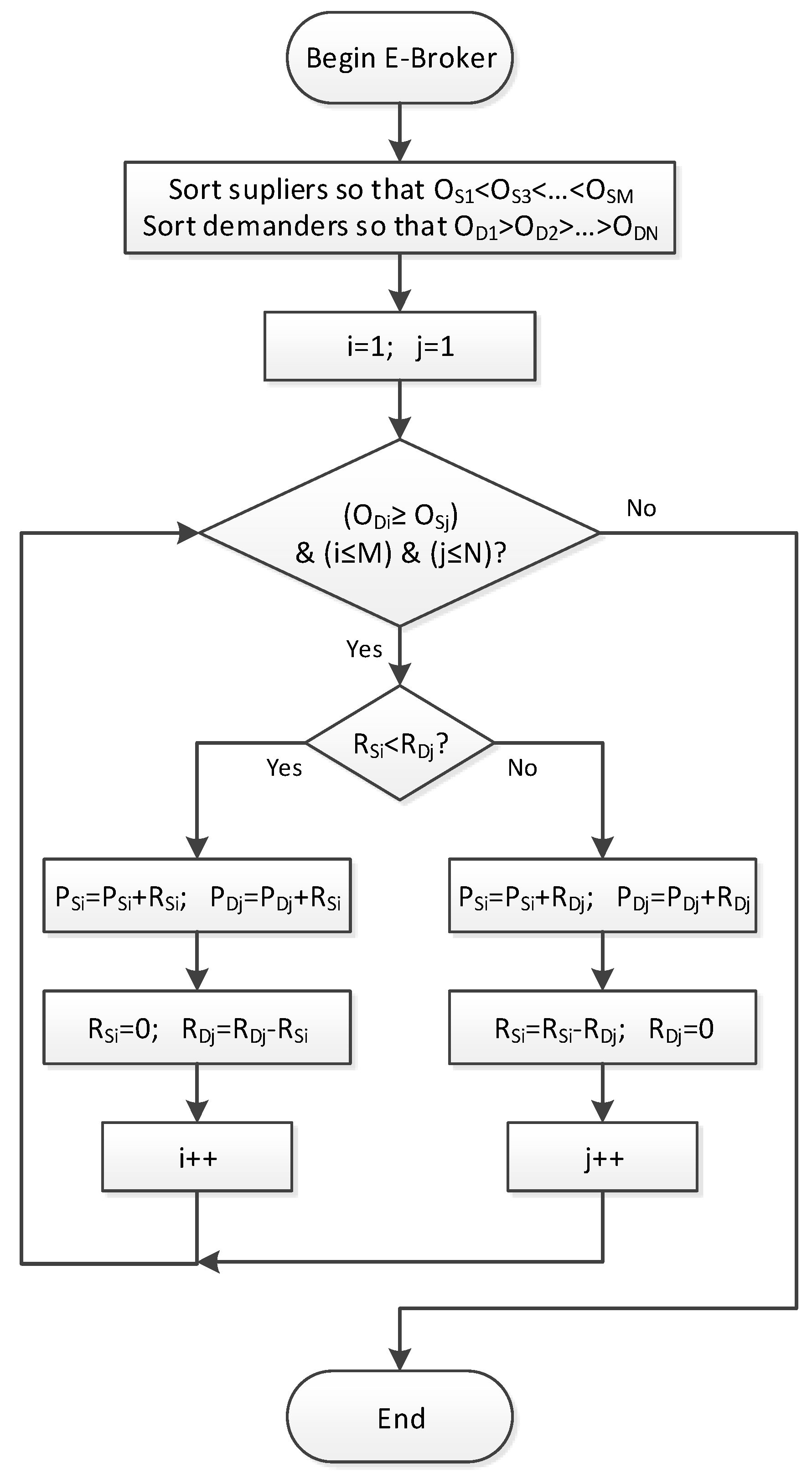
Suppliers and demanders are sorted according to their priority values. Higher priorities are represented with greater priority values for demanders and with smaller values for suppliers. In addition, for an exchange between supplier i and demander j to occur, the priority value of the demander (O
Dj) must be greater than or equal to that of the suppliers (O
Si). This is similar to a market auction where priority values act as prices.
Table 1 shows the sorted suppliers and demanders, their priority values and whether a combination is allowed (A) or forbidden (X).
Devices are checked in priority order and each demander is searched for a supplier with equal or lower priority that has power available to feed it. This way, the algorithm calculates the power each supplier must provide P
S1…P
SM and each demander must receive P
D1…P
DN, having a balance between the total power delivered and received.
Figure 4 summarizes the E-Broker Auction Algorithm.
Since the power requests for the PV facility and the loads were based on the actual power of these devices, and the distribution grid is not controlled from the microgrid, only the battery power needs to be applied. To do so, the inverter connected to the battery is commanded to charge (or discharge) the battery at a certain power rate. The net power the battery must absorb is P
Bat, which is calculated from the power values selected by the E-Broker algorithm as shown in
Figure 3.
A detailed example is provided for better clarity.
Table 2 shows the power requests (R), as well as the final powers (P) each device must provide or receive.
For this example, the battery can charge or discharge at 5 kW and at the point of the shown execution of the RT cycle SOC is lower than SOCb. Therefore, Bat A makes a request as a demander to get to SOCb: 3 kW, which is enough to get to SOCb by the next cycle. Bat B requests to keep charging with the remaining charge power (2 kW) in case there is an excess of PV power. Bat A also requests to discharge at up to its maximum rate (5 kW) if needed.
The power request of Grid A is given by Pb which, in this example, is 8.5 kW. Due its priority, the power of Grid B will only be used if the power required by the load is greater than the sum of the powers of the PV facility, Grid A, and the battery. This will help preventing grid power peaks greater than Pb.
The E-Broker algorithm starts by checking the first demander (the Load) and the first supplier (the PV facility). It verifies that the priority of the demander is greater than the priority of the supplier, so the exchange is allowed. The load request is greater than the PV facility request, so all the power of the PV facility is assigned to the load.
The PV facility has exchanged all its power, but the Loads still request to receive 8 kW more. The E-Broker algorithm searches for the next supplier with a power request greater than 0: Grid A. It is verified that the priority of the loads is still greater than that of Grid A. Thus, the remaining power that was missing from the load is exchanged, 8 kW, leaving Grid A with 0.5 kW available to assign.
The algorithm confirmed that the priority of the next demander (Bat A) is greater than that of Grid A. The exchange is possible, so the remaining 0.5 kW of Grid A are assigned to Bat A. The remaining 2.5 kW of Bat A must stay unassigned since all other suppliers have greater priority values. There are no other demanders whose priority is greater than those of the remaining suppliers, so no more power can be assigned.
In the end, the PV facility provides 4 kW (as originally measured), the load consumes 12 kW (as measured), the battery is commanded to charge at 0.5 kW and the grid provides the difference: 8.5 kW. Please note that even though the E-Broker algorithm considers power transferring in pairs of devices (a supplier and a demander) the actual route of the power may be different. For example, the 0.5 kW used to charge the battery may actually be coming from the PV facility. The E-Broker only decides how much each device exchanges, not which device it is exchanged with.
2.2. Implementation and Test Description
A test bench has been built to validate the proposed method, as shown in
Figure 5. Here, a 20-kW PV system and a 10-kWh-energy and 5-kW-power battery are employed. The load is emulated using a revertible power source and an inverter controlled by a raspberry pi (model 3B). This load emulation system is programed to consume power according to historic data from previous days.
The proposed method is distributed among a programmable logic controller (PLC) and a personal computer (PC) acting as a server, which communicate with one another using the message queue telemetry transport (MQTT) protocol.
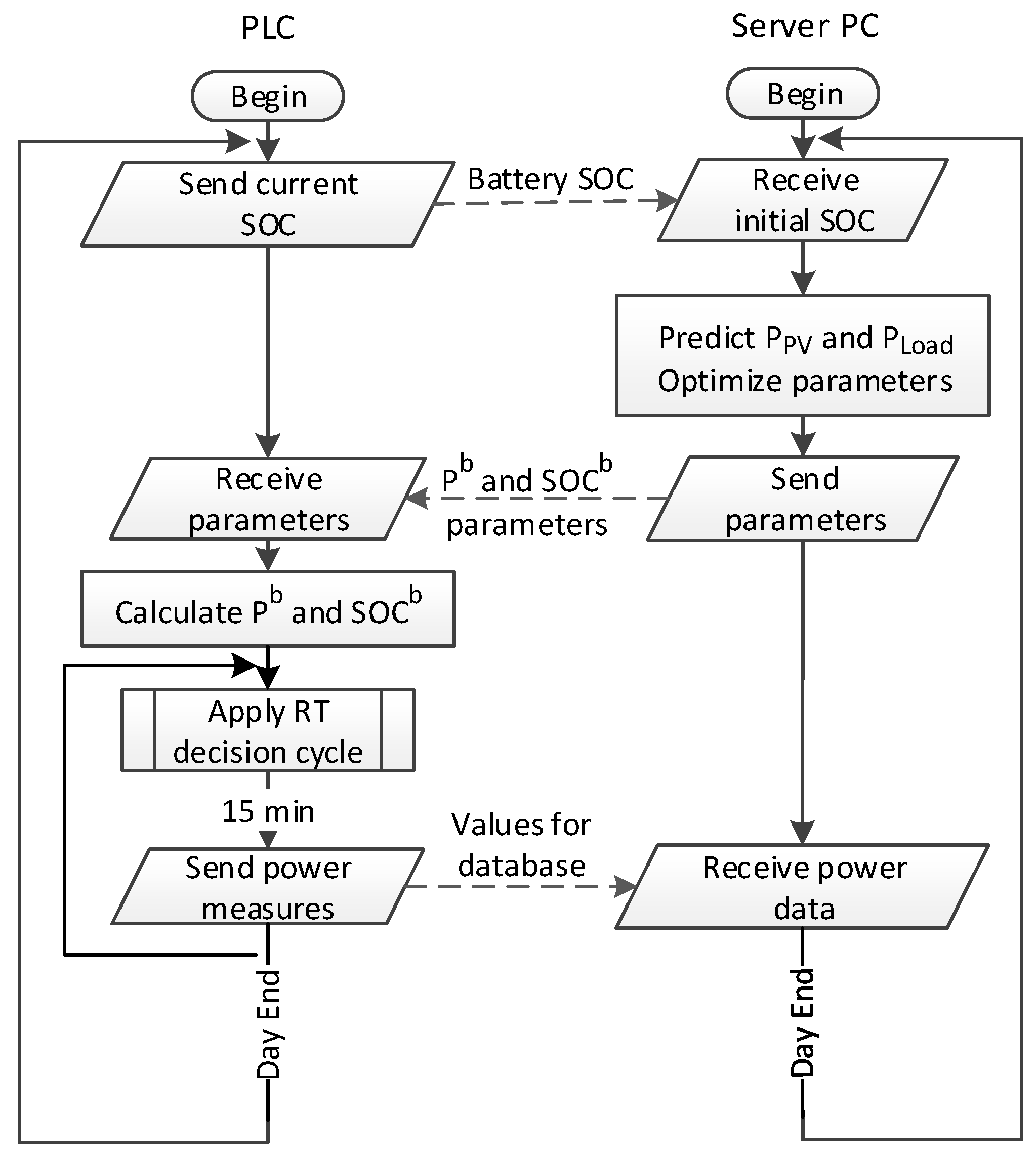
As shown in
Figure 6, the server PC runs the aforementioned prediction and optimization at the beginning of each day. After each optimization, the PC server sends to the PLC the necessary parameters so that the latter can reconstruct P
b and SOC
b through linear interpolation.
Using this information, the PLC receives the measured power values of the load and PV systems, runs the RT decision cycle shown in
Figure 3 and
Figure 4, and commands the battery inverter to charge or discharge the battery accordingly. This RT decision cycle is executed every 5 s.
Every 15 min, the PLC reports the average PV power production, load consumption, and battery SOC for that time period. This information is stored in a data base to train the ANNs, as well as to evaluate the results of the proposed method.
The tests have been performed considering days independently. Since the power cost can only be evaluated for periods of at least one month, the grid electricity bill has been calculated considering 30 equal days. The prices used and their corresponding time periods are shown in
Table 3. The objective function has been calculated considering the Contracted Power is 10 kW.
Among the referenced publications for optimal scheduling, [
17,
22] are the newest ones. The method from [
22] aims for the same purpose and considers some real-time control. The method from [
17], on the other hand, intends to control a whole distribution grid and would be harder to adapt. Thus, the proposed method is compared to [
22], which can be considered the state of the art. Since the method from [
22] did not originally consider PV generation, an additional adjustment has been made to it: whenever the PV generation is greater than the load power, the battery will attempt to absorb the power excess in the same way it would attempt to prevent power peaks. This can be understood as the battery avoiding a negative power peak. This adjustment always produces a better result as otherwise this extra power would be unused. The simulation is run for the same day, with the same power values for the PV generation and load consumption, and the method from [
22] is provided the same prediction as the proposed method had at the beginning of the day, so that they can be compared under the same conditions.


