Detection and Identification of Demagnetization and Bearing Faults in PMSM Using Transfer Learning-Based VGG

Abstract

Predictive maintenance in the permanent magnet synchronous motor (PMSM) is of paramount importance due to its usage in electric vehicles and other applications. Recently various deep learning techniques are applied for fault detection and identification (FDI). However, it is very hard to optimally train the deeper networks like convolutional neural network (CNN) on a relatively fewer and non-uniform experimental data of electric machines. This paper presents a deep learning-based FDI for the irreversible-demagnetization fault (IDF) and bearing fault (BF) using a new transfer learning-based pre-trained visual geometry group (VGG). A variant of ImageNet pre-trained VGG network with 16 layers is used for the classification. The vibration and the stator current signals are selected for the feature extraction using the VGG-16 network for reliable detection of faults. A confluence of vibration and current signals-based signal-to-image conversion approach is also introduced for exploiting the benefits of transfer learning. We evaluate the proposed approach on ImageNet pre-trained VGG-16 parameters and training from scratch to show that transfer learning improves the model accuracy. Our proposed method achieves a state-of-the-art accuracy of 96.65% for the classification of faults. Furthermore, we also observed that the combination of vibration and current signals significantly improves the efficiency of FDI techniques.

1. Introduction

The permanent magnet synchronous motor (PMSM) is a kind of motor with excellent dynamic performance and high reliability. PMSMs are an important asset in transportation, industry automation, and aerospace where these motors drive a diversity of loads. PMSMs are continuously involved in highly variable operation regimes and often subjected to transients (load variations, repeated start/stop, and acceleration/deceleration) [1]. During the operation of PMSMs, performance degradation or even failure will inevitably occur, which will seriously affect the reliability and safety of the whole system [2]. Different types of faults such as bearing fault (BF), winding insulation breakdown, eccentricity, and irreversible demagnetization fault (IDF) can occur in a PMSM [3]. BF and IDF are the most commonly occurring faults where BF itself accounts for over 40% of all motor faults [4,5]. The potential reasons for BF are excessive temperature, improper lubrication, corrosion, contamination, improper mounting, and fluting [6]. Whereas the IDF occurs due to high operational temperature, severe field-weakening, the reverse magnetic field of winding short faults, and physical damage [7,8]. Such failures have severe implications on the performance of the motors which can be responsible for serious loss and may lead to catastrophic accidents [9,10]. Therefore, early diagnosis of such faults is required to ensure safety, enhance reliability, expedite the unscheduled maintenance, and decrease the downtime of the motor.

Fault detection and identification (FDI) in the electric motor has been substantially studied so far. FDI can be classified into model-based, signal-based, knowledge-based, and the combination of these techniques [11,12]. Model-based FDI requires an accurate mathematical model of the machine and signal-based FDI is highly dependent on machine operating point [12] while knowledge-based FDI is a data-driven technique that depends on a big amount of experimental dataset to organize the fault classes. Consequently, data-driven FDI techniques are appropriate for highly nonlinear systems with the unknown model or specific signal patterns [13]. Recently, the rapid growth in the smart system industry made the collection of large datasets easier, which provided new opportunities for the knowledge-based FDI techniques to fully utilize the available big data for complex systems.

Machine learning (ML) is one of the popular techniques to implement data-driven FDI. Support vector machine (SVM) was the first ML-based technique that was initially applied to diagnose faults in the late 1990s [14]. Fuzzy classifier has the ability to represent different faulty features into fuzzy sets and classify it based on fuzzy rules. A new decision tree-based fuzzy classifier technique was proposed for rolling bearing fault detection [15]. Multiple discriminant analysis and ANN is applied to diagnose the broken rotor bar in the induction motor [16]. Furthermore, Park’s vector approach-based ANN method is proposed for the diagnosis of electrical faults in induction motor [17]. However, the efficiency of ML-based models is heavily dependent on the quality of the feature extraction process that is hard-coded by human experts. Moreover, the meaningful feature selection process is cumbersome in ML as the features selected for a particular type of fault may not be suitable for another fault.

Since the last two decades, deep learning (DL) has risen as a very effective method for FDI in different fields [18,19,20,21] and it has proved its effectiveness in automatically extracting features from raw data. Thus, it can alleviate the dependence on the diagnostic knowledge of human experts (extraction and selection of meaningful features). Additionally, DL can form a relationship between experimental data and the type of fault using a multilayer architecture. Several DL techniques have already been used for the fault diagnosis, such as convolution neural network (CNN) [22], deep belief network (DBN) [23], sparse auto-encoder [18], stacked denoising autoencoder [24], and sparse filtering [19]. CNN is one of the most effective DL methods which has been widely used in the fault diagnosis as it extracts meaningful hierarchical features [22]. The most commonly available data is the time-domain signals. Therefore, the one-dimensional (1-D) CNN has been investigated on the real-time motor fault diagnosis [20]. However, the commonly used time-domain signals (stator current and vibration signals) can either be affected by noise or may not provide sufficient information in some operating areas which might lead to misdetection [21]. Furthermore, DL methods are dependent on a significant amount of data to optimize the classification weights for predictions while the generation of a huge amount of faulty machine data is cumbersome in the FDI domain. Moreover, DL networks also have the tendency to easily overfit in case of small datasets with a higher number of trainable parameters. Therefore, DL approaches need specific architectural improvements before applying it in the FDI domain. Moreover, most of the data-driven FDI techniques in the literature focus on BF fault and use vibration signal for fault diagnosis [18,19,20,21,24,25,26]. The frequency-domain signal of stator current is also used for the diagnosis of BF [23]. However, each of the signals has its own limitations such as the vibration signal is extremely sensitive to noise while the stator current signal is prone to be affected by other types of faults, such as eccentricity fault and load variations [27]. Kim et al. explain that the harmonics generated by a fault in the stator current can be influenced by controller action in a closed-loop system [28]. Therefore, these issues raise the probability of the false alarm by using either a vibration signal or a current signal alone.

This paper proposed a new method for the FDI of IDF and BF which not only overcomes the above-mentioned limitations of motor data but also alleviates the complexities of the DL approaches.

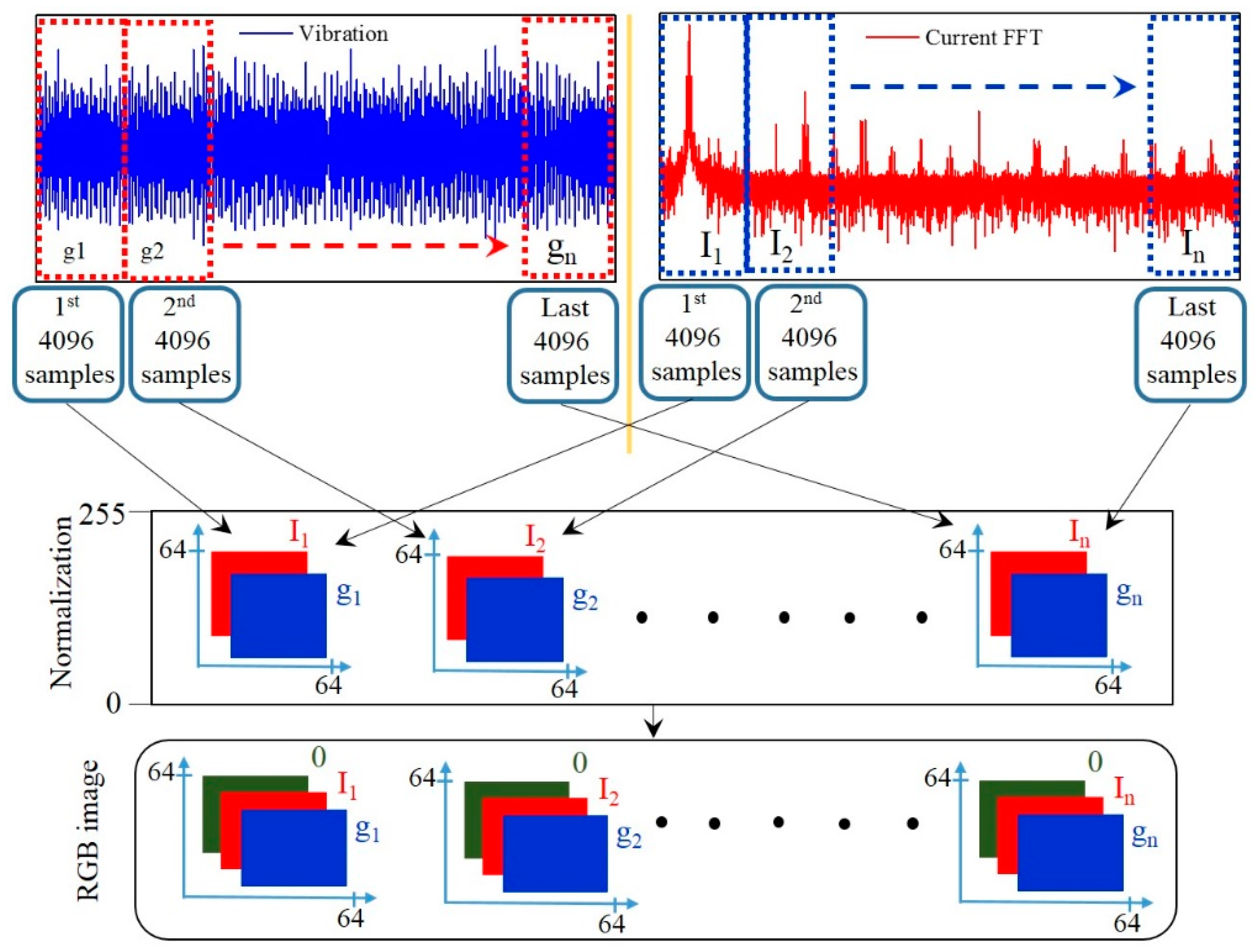
The time-domain signal of vibration and the frequency domain signal of the stator current together are used for the diagnosis of IDF and BF using the deeper architecture of visual geometry group (VGG) with 16 layers. The usage of multiple signals together makes the FDI more robust. Transfer learning technique is used to overcome the problem of overfitting while training VGG-16 using a small dataset. Furthermore, a new technique for data preprocessing is proposed, which converts the two-dimensional current and vibration signals into RGB images without knowing any parameter. This is a simple signal processing method that does not require a higher experience. An experimental evaluation of the proposed model for the combination of current and vibration signals is compared with their individual usage for classification of faults. A comparison between our proposed model with pre-trained and without pre-trained weights are provided for analyzing our hypothesis that transfer learning helps in increasing the efficiency of the model. The proposed method was compared with the other existing techniques for verification.

The rest of the paper is organized as follows. Section 2 presents the preliminaries of the related work. Section 3 provides the detail of the IDF and BF modeling, analysis, and data acquisition. The methodology of the proposed FDI is presented in Section 4. Section 5 presents the results and Section 6 presents the discussion followed by the conclusion.

2. Preliminaries

A complete solution to a motor fault diagnosis problem can be divided into three steps: fault detection, fault type classification, and fault severity prediction. Among all kinds of motor fault diagnosis methods, DL model is usually unable to build an end-to-end model due to its difficulty in obtaining training data and poor anti-noise ability. It needs to extract artificial features and then use the DL model to realize fault diagnosis [29]. However, the DL model has strong non-linear fitting ability and can be used as a part of the diagnosis method for feature preprocessing and other operations. In addition, most of the stator current-based PMSM fault diagnosis methods have difficulties in fault severity prediction, so to express the main work of this paper more clearly, in this section, a brief introduction to CNN and VGG methods is given.

2.1. Transfer Learning

Transfer learning (TL) is a technique where the knowledge of an already trained model for a specific task is transferred to another model developed for another task. The knowledge of a pre-trained model on a big dataset is reused at a starting point of a model to be trained for another task [30]. In DL, the TL approach became popular and widely used as the initial point on natural language processing and computer vision problems. TL provides a huge jump on the problem which requires vast time resources and computation to develop neural network models using the knowledge learned by the related problems. However, in machine fault diagnosis, the availability of long enough data at all operating conditions is huge. Because it is not possible to operate the faulty machine for a long time that covers every operating condition. Such small datasets are not enough to optimally train complex networks like CNN. Therefore, using a CNN-based network for fault diagnosis may easily overfit.

In TL, first, a base network is trained on a base dataset, and then the learned features are repurposed, or the knowledge learned at base dataset is transferred to another network to be trained on a target dataset to perform the required classification task. This process will tend to work if the features are general. Figure 1 shows the distribution of a basic network. Every network of CNN consists of convolution layers that are used for the feature extraction and the fully connected layers (FC) that are used for the classification purpose. In our fault diagnosis problem, we do not share the classification part of the pre-trained network with our task. Thereby, we removed the classification part of the model and use only the feature extraction (convolution layers) part of the network. The feature extraction part of the model is focused to look at patterns, lines, and textures of the images that are required to do to extract meaningful information. We used an optimally pre-trained feature extraction as a starting point for our model and attached our own classification network to it for re-training.

2.2. CNN-Based VGG

Convolutional neural network (CNN) is widely used in a wide range of applications such as video recognition, recommender system, image recognition, and natural language processing [30]. CNN uses shared convolutional kernels to extract features from input. The shared convolutional kernels save a lot of memory and computational cost. A CNN model is divided into two main parts, which are feature extraction and classification. The output of shared convolutional kernels is called features used as input for the classification part. Feature extraction part requires an enormous amount of data to optimize and extract meaningful features. Our data is not so big; therefore, we start the training of our feature extraction model from an already trained model that is optimized on the ImageNet dataset. In this way, the data requirement and optimization issues can be alleviated.

This study used a pre-trained VGG model [31] as a training starting point for the task and these parameters are optimized during the training accordingly. VGG model is one of the best performing models on ImageNet classification challenge [32], which consists of approximately 14 million images belonging to 1000 classes. VGG network achieved a benchmark accuracy of 92.7% on the ImageNet classification task. The simplest model of VGG with sixteen layers is selected for this study. There can be multiple types of layers such as convolution, fully connected, dropout, pooling, etc. Convolutional layers have trainable weights (filters) typically of 3x3 size that are used for convolution operation in a layer and extract pixel-wise information. Dropout layers are used to prevent the model from overfitting by randomly setting some of the output of the layer to zero with a probability of (p-dropout rate) and let the model learn this noisy data. Dropout is used in the training phase only. Pooling layer applies a discretization process to reduce the size of the input. Pooling operation is typically performed after the non-linearity function. There can be many non-linearity functions such as sigmoid, ReLU, PReLU, etc., but ReLU is the most used one. ReLU is computationally efficient and it helps in alleviating the gradient vanishing problem. Finally, the fully connected (FC) layer is used to perform the classification task. FC layers receive the feature maps from the feature extraction part for the classification task. A neuron in the FC layer is connected to every other activation neuron in the subsequent layer which makes them computationally very expensive; therefore, we use a smaller number of FC layers in the network. In our solution, we use a pre-trained convolution base with a personalized classification part including the FC classifier and dropout layer for regularization.

3. Fault Analysis and Data Acquisition

Any kind of fault causes several variations in the electrical and mechanical parameters of PMSM such as current, voltage, magnetic flux, torque, and vibration. Whereas the current and the vibration signal carry more valuable information. Although these two signals separately have been applied for FDI of winding related faults, IDF, and BF. However, their reliability is often limited by noise, other types of fault, and controller action in closed-loop control. In this paper, we propose a novel approach for FDI, which combines the analysis of both signals for robust detection of faults. To the best knowledge of authors, this is the first study that analyzes the confluence of both signals classification of healthy, IDF, and BF conditions of PMSM. The detail of both types of faults i.e., IDF and BF are given below.

3.1. Irreversible Demagnetization

IDF is one of the major hurdles for PM type machines in achieving high power/torque density while operating in harsh environments. High operating temperature, vibration, physical damage, and aging cause permanent reduction in the remanence magnetic flux density of the embedded permanent magnets (PMs) in the rotor of a PMSM which is called IDF [33]. To realize the IDF in the experiment, reduced size PMs are designed and inserted in the rotor of the PMSM, as shown in Figure 2. Nonmagnetic material is placed with reduced size PMs to avoid unwanted movement during operation. Experiments are conducted under various severities of IDF and the vibration and the frequency spectrum of the stator current signals are obtained at various speeds and load as mentioned earlier. The combination of different IDF severities are shown in Figure 2. These combinations of reduced magnets are used for single-pole, two poles, three poles, and all six poles. The real reduced magnet inserted in the rotor of the PMSM can be seen in Figure 2b. The data for all these cases are recorded for the same duration of time and the same operating conditions.

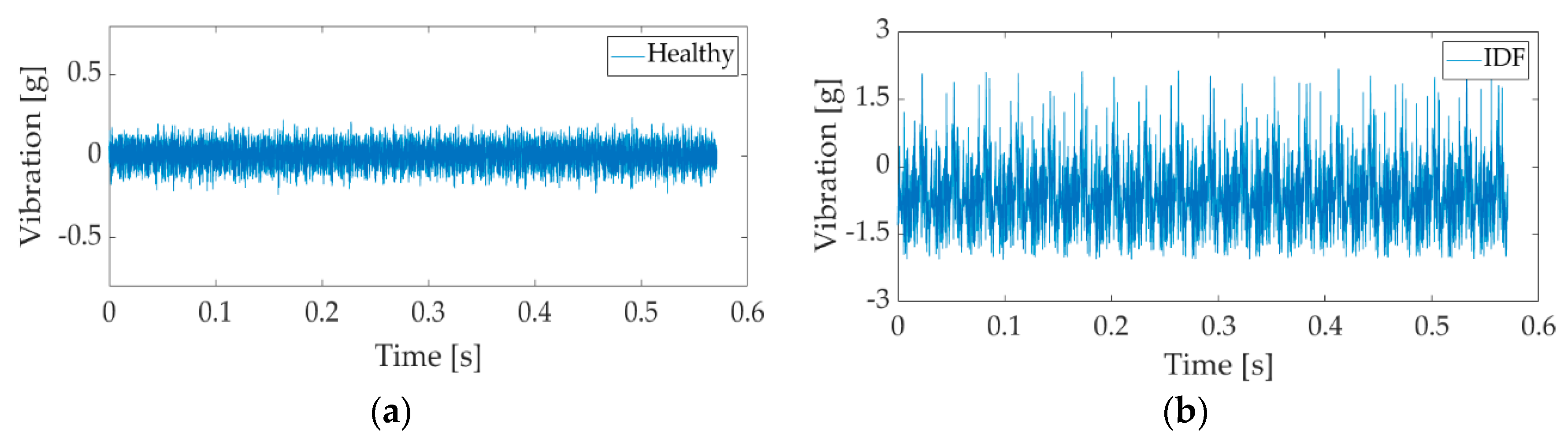
The experimental result of the vibration of the benchmark machine under healthy and IDF is shown in Figure 3. It can be seen that in the case of the healthy machine the vibration is very small and with a uniform pattern. However, for IDF, different pattern and increased magnitude in the vibration signal can be seen. Similarly, the experimental result of the stator current is also shown in Figure 4. The frequency spectrum of the stator current was obtained at rated load and speed under healthy and single pole IDF. It can be seen that the IDF significantly increases the second and fourth order harmonics while suppressing the fifth harmonic for the benchmark PMSM as shown in Figure 4b. Other higher order harmonics are also clearly affected by the different severities of IDF. A clear difference in both vibration and current signal due to IDF can be seen. Such differences can be used as a fault signature and can be used for the detection and identification of IDF.

3.2. Bearing Fault

Bearing fault is the most frequently occur fault in the electric motor which accounts for above 40% among all types of faults. Generic deep-groove ball bearing consists of the outer race, inner race, and balls, as shown in Figure 5a. Lubricant is applied to the rolling elements of the bearing. As mentioned above there are several reasons for BF. Normally, the machines are carefully designed and operated to avoid BF. However, even in a very vigorous system, the gradual degradation of bearing due to electrical stress can still lead to BF, which needs to be detected at its early stage to avoid further damage. With inverter controlled PMSMs, the high switching frequency leads to common-mode voltage and bearing current [34]. The flow of current through the surface of the bearing increases the Joule loss, which raises the temperature [6]. The rise in temperature affects the impedance and the viscosity of the lubricant in a bearing; thus, the flow of the bearing current via the motor shaft increases. When the bearing is exposed to high current density (more than 0.6A/mm²) for a long time, the bearing is degraded and damaged like fluting and pitting occurs on the surface of bearing. These mechanical strains cause increased vibration and acoustic noise.

In real scenario, when the inverter fed machine is operating, there is a small current due to parasitic capacitance, which always circulates through the shaft and bearing and slowly damages the surface of the bearing as explained earlier. The same method is performed using a higher current (accelerated process to damage the bearing) to realize the bearing fault. In this method, the electrical stress is applied by passing a high current through the bearing during the operation of the machine. 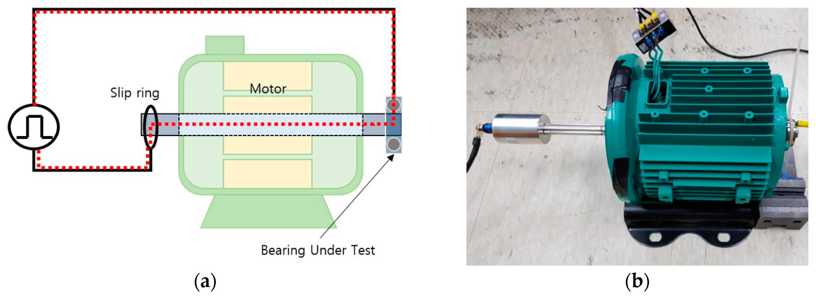Figure 5b shows samples of bearings damaged using the electrical stress. The schematic diagram of the process and real experimental setup, which is used for applying electrical stress to damage the bearing is shown in Figure 6. The bearings were kept under stress for different times (10 minutes to 1 hour). The level of damage is directly proportional to the stress duration. Figure 7a,b shows the microscopic view of the surface of the outer race of the healthy and damaged bearing, respectively. The damage caused to the outer race of the bearing is due to the stress (30 minutes) caused by the passing of higher direct current. The experimental result of the vibration signal under bearing fault is shown in Figure 8. It can be seen that the pattern and the magnitude of the vibration is completely different to that of the healthy machine (Figure 3a). Furthermore, the frequency spectrum of the stator current under bearing fault is given in Figure 9. The BF not only increases the fundamental component but also causes a number of additional harmonics when compared to a healthy machine. These additional harmonics in the entire spectrum of the current and also the vibration cannot be extracted manually. Therefore, the deep learning-based methods are extremely suitable to automatically extract all these features and use it for the optimal classification of faults. Different severities and types of fault cause different patterns; hence, they can be easily classify using deep learning.

3.3. Experimental Setup

In this section, the detail of the experimental setup used for obtaining the training and testing data for the implementation of the proposed method is discussed. The data was obtained by performing experiments on a medium size (400-watt) interior type PMSM. Figure 10 shows the experimental setup used in this study. The detailed parameters of the benchmark PMSM is given in

Table 1. Parameters of the benchmark PMSM.

Parameter	Value	Parameter	Value	Parameter	Value
Rated power (watt)	400	Ld (mH)	0.92	DC bus voltage (V)	60
Rated speed (rpm)	3500	Lq (mH)	1.35	No. of turns/phase	72
Rated current (Arms)	10.32	Resistance (ohm)	0.07	PM type	NdFeB
Rated Torque (Nm)	1.1	Poles	6	Slots	9

. A conventional field-oriented control (FOC) drive was used to operate the motor under healthy and fault conditions. Tms320F28335 DSP board is used for the control and operation of the inverter. The switching frequency was kept at 10 KHz. The stator current signal was collected using the Lecroy 44MXs-B oscilloscope at different loads and speeds. Dytran 3093B1 accelerometer was attached to the body of PMSM to record the vibration signal. The obtained data were recorded under healthy conditions, IDF, and BF. The data were recorded at different speeds (2000 rpm, 2500 rpm, 3000 rpm, and 3500 rpm) and different loads (0%, 25%, 50%, 80%, and 100% loads). All the data were recorded at a 50 kHz sampling rate. In the case of the vibration signal, a Butterworth filter was applied to reduce the noise in the raw signal.

4. Methodology of the Proposed FDI

There are three major steps to implement the proposed algorithm. First is data acquisition, second is signal to RGB image conversion and the last one is training and testing. Figure 11 shows the block diagram of the overall FDI process which describes the information flow between multiple blocks. In this section, the details of each step are presented.

4.1. Signal-to-Image Conversion Method

Different DL-based methods have different formats of input signals. Therefore, the prepossessing of the raw signal obtained from simulation and experiments in the DL based FDI is the most crucial step because the robustness and accuracy of the FDI are completely based on the training and validation dataset. In this study, an effective data processing method is developed. The method of signal to RGB image conversion used in this paper is shown in Figure 12. In order to obtain the Z × Z image, the raw data of vibration signal and frequency spectrum of stator current is divided into equal size of segments with each segment consist of Z² samples. The segments of vibration and current signals are combined from start to end, sequentially. If a segment from vibration signal “g” and a segment from current frequency spectrum “I” have Z × Z size, then a point in the 2D matrix is denoted by P(x, y), where x = 1, ..., Z, y = 1, ..., Z. To obtain a three-channel image (RGB), the third dimension of zeroes is padded with the image. In an RGB image, the point P(x, y) represents the pixel strength given by equation.

$$P(x,y)=round\left\{\frac{(P(x,y)-Min(Z))}{Max(Z)-Min(Z)}\times 255\right\}$$

(1)

Using Equation (1), the pixel values are normalized from 0 to 255, which is the minimum and maximum limit of a pixel value in an RGB image. In this study, a 64×64 image size is used. Figure 13 shows the converted images of the vibration and current frequency spectrum signals of the healthy machine, IDF, and the BF under no-load and full load conditions. The main advantage of this data processing method is that it converts all the points of a raw signal to images in sequence; thus, there is a minimum loss of original information. Furthermore, this method does not require any predefined parameters or features.

4.2. Data Augmentation

Data augmentation technique is used to artificially expand the dataset size by a modified version of the original dataset points. It adds diversity in the input data for model training and makes the model robust against unseen data. We applied three different types of data augmentation techniques such as vertical flip, horizontal flip, and random crop to the training dataset only. Vertical flip is applied with a probability of having a threshold of 0.5. Every time a random image is selected for training, we attach a random vertical flip probability to it. In case the probability number is higher than the threshold, a vertical flip version of the image will be used for training. Randomized horizontal flip probability with a threshold of 0.5 is also attached with the image and a modified horizontal flipped version of the image is used if the probability is higher than the threshold. In the case of the random crop, first, every image was padded with four rows on each side of the image dimension and then we randomly crop a 64×64 image from this increased image. By applying this selected data augmentation, the training data is changed in every epoch while increasing the robustness of the model.

4.3. Proposed Deep Learning Model

CNN, a relatively complex model, has achieved an outstanding performance on very difficult recognition tasks but it requires a huge number of data samples for optimizing the weights. Researchers have created larger datasets for specific tasks for CNN models training and released these trained models (VGG, GoogleNet, ResNet, etc.) to the general public for future research. Nowadays, these pre-trained models are being used for several other tasks where the collection of the larger dataset was not possible or not existed by adopting the TL technique. Several strategies are in practice for performing TL to reuse the knowledge of a pre-trained model for feature extraction from an image. Fault diagnosis is one of the perfect examples of the task where the collection of larger training is not feasible therefore, TL can help to achieve better accuracy. We selected VGG with sixteen layers (VGG-16) because it is one of the smallest pre-trained models available for TL, as larger models can easily overfit the smaller training data. The architecture of VGG-16 is presented in Figure 14. The proposed architecture consists of pre-trained convolution layers with a customized classification part, included a fully-connected classifier and a dropout layer for regularization.

4.4. Training

The proposed neural network takes a 64 × 64 pre-processed RGB image as an input and classifies it into three different classes (Healthy, IDF, and BF), which indicate the faults that need to be diagnosed. Since in the proposed model the ImagNet-based pre-trained VGG-16 model was used, it therefore required merely training of the classification layers, which consisted of dense and dropout layers. The convolution part of the VGG-16 model was run by our own training dataset and obtained the output vectors from the last layer, which was then used as the training input for the classification part of the proposed model. Since our classification task is based on a multi-class classification problem, the categorical cross-entropy loss function, which is also known as “Softmax” loss, was used in the classification in the proposed model. This function contains the Cross-Entropy loss and the Softmax activation that evaluate the rate of error. The Categorical Cross-Entropy (CE) is given by [35]

$$CE={\displaystyle \sum _i^C{t}_i}\log (f{(s)}_i)$$

(2)

In Equation (2) the t_i represents the ground truth and f(s)_i represents the standard Softmax function. The Softmax function for a given class S_i can be written as

$$f{(s)}_i=\frac{e^{si}}{i^C{e}^{si}}$$

(3)

where S_j represents the scores achieved by the network for each class in C.

Since there are three different classes, any sample can be part of one of the classes. The number of output neurons in CNN is always equal to the number of classes which are obtained in vectors or scores. The vector t (ground truth) is a one-hot vector with a positive class and C-1 negative classes (zeroes); thus, the CE can be written as

$$CE=-\log \frac{e^{s_p}}{{\displaystyle \sum _i^C{e}^{s_j}}}$$

(4)

where S_p is the score for the positive class. The stochastic gradient descent algorithm was used with Nesterov moment (0.9). The optimization algorithm aims to find optimal weights, maximize accuracy, and minimize the corresponding error. The optimizer continuously updates the weights of the neurons using back-propagation. The optimizer evaluates the rate of change of the loss function for each weight and subtracts it from the net weight.

The proposed method is implemented using the “PyTorch” library in the “Google CoLab” environment with a single GPU. Three different classes such as healthy, IDF, and BF are considered. We made a total of 1428 images whereas 1140 images were randomly chosen for training with equal ratio from each class and 288 images were used for validation. The number of epochs was set as 200. Stochastic gradient descent algorithm was used with Nesterov moment (0.9) and the learning rate was used as 5e⁻⁴. The batch size during training, validation, and testing were set as 50, 20, and 20, respectively.

5. Results

The discrepancies in classification were analyzed, which are the differences between the actual classifications and the classification that were carried out by the classifier to evaluate the performance of the proposed solution. The accuracy is calculated using Equation (5).

$$Accuracy=\frac{TP+TN}{TP+TN+FP+FN}$$

(5)

where TP is true positive, TN is true negative, FP is false positive, and FN is false negative.

The results show that our model classifies the faults with higher accuracy and does not over fit the training data. The model is generalized enough, and the generalization property of the proposed model is explained in the next section. By referring to Figure 15, it can be seen that there is no specific pattern in the images obtained in all three cases except the no-load healthy condition, which states that our data is not linearly separable and it requires multi convolutional layers to extract the deeper features for classification of the data. Linearly separable data does not require many convolutional layers and complex networks easily over-fit it in a lesser number of epochs. However, in real applications, the vibration or stator current data under various operating conditions is not linearly separable.

Table 2. The test set accuracy using transfer learning (TL)-based model and model training from scratch.

Training Method	Average Accuracy (%)
Transfer learning	96.65
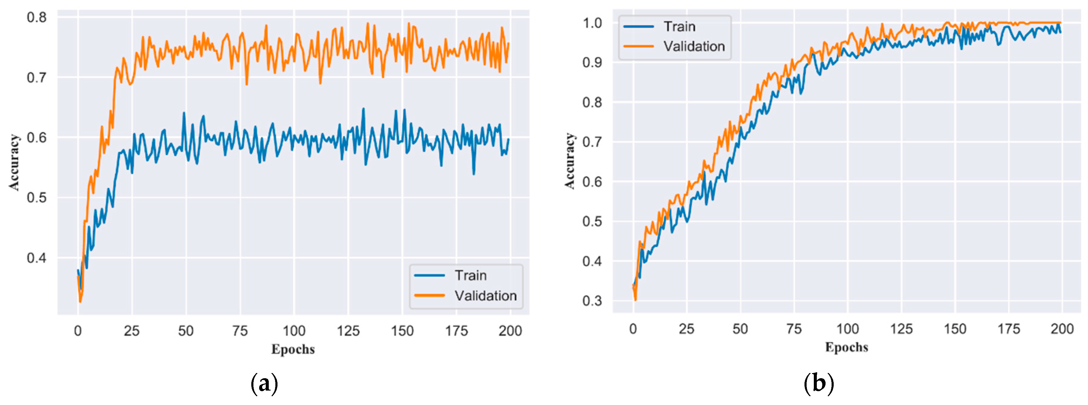
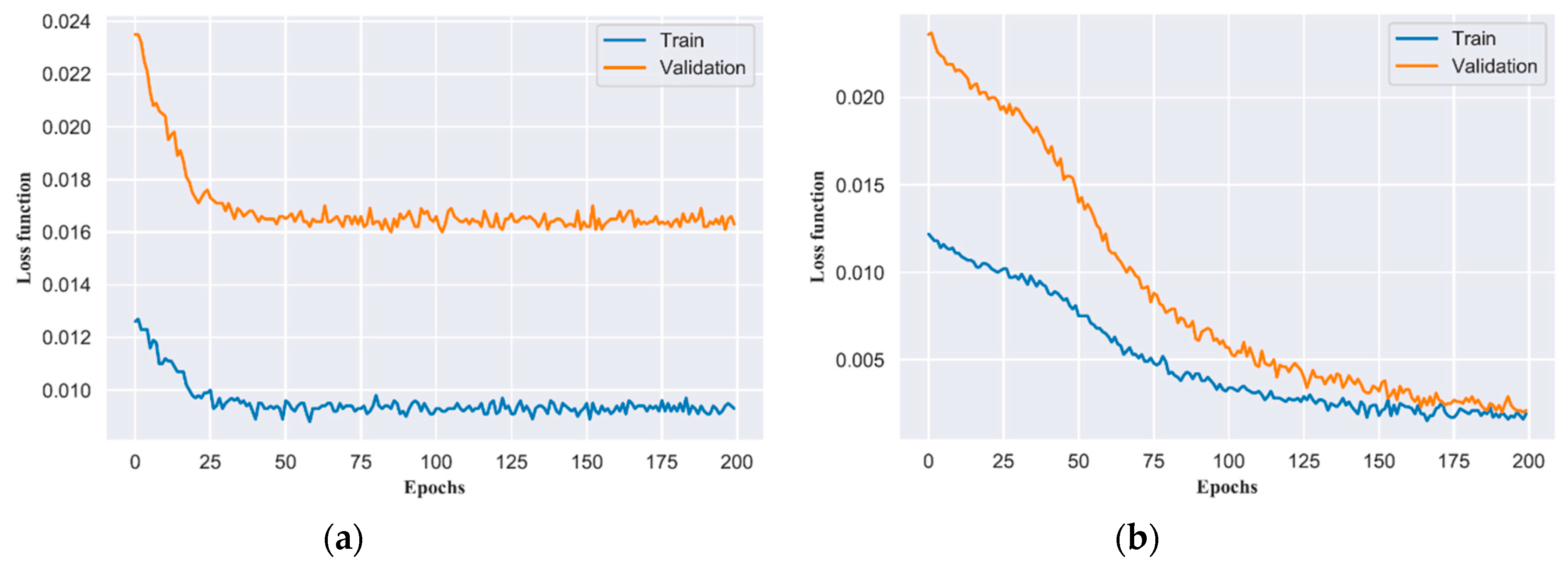
Without Transfer learning	67.32

shows that our model achieved an accuracy of 96.65% accuracy rate with pre-trained weights, whereas it achieved 67.32% accuracy with training from scratch on the test set. In order to show the training process of the model and over-fitting issue, the training and validation loss of the model with its achieved accuracy at every epoch is plotted. This also shows the learning curve of the model. Training and validation accuracy for the model trained from scratch and pre-trained are plotted in Figure 15a,b while training and validation loss for both models are plotted in Figure 16a,b, respectively. Figure 15b shows that the model is gradually learning the data complexities and achieves high accuracy. There is not much distance between training and validation accuracy which states that the model is neither over-fitted nor under-fitted while this distance is visible in Figure 15a. Furthermore, we have evaluated our model for current and vibration signals individually and the results are given in

Table 3. Validation accuracy comparison for current (I) and vibration (g) as input individually and combined.

	Input Signal Type
	Current	Vibration	Current and Vibration
Accuracy (%)	33.3	44.79	96.65

. The results explain that the combination of signals significantly improve the FDI accuracy.

In order to compare the performance of the proposed technique the same training data was tested on support vector machine (SVM), linear discernment analysis (LDA), and quadrature discernment analysis (QDA), which are machine learning methods often use for classification. SVM is considered the best machine learning method for nonlinear data classification. Because these methods are in the domain of machine learning, they require manual feature extraction from the data. The Haralick texture consists of 13 different features that are first extracted from each image [36]. After feature extraction, the classification was performed using the SVM, LDA, and QDA for healthy, IDF, and bearing fault data. The accuracies of these three methods are compared with the VGG in

Table 4. Comparison of the accuracy with other techniques.

	Type of Method
	SVM	QDA	LDA	VGG
Average Accuracy	67%	70%	85%	96.56%

. The detailed result of the all the methods can be seen in the form of confusion matrices in Figure 17. The LDA shows a better average accuracy of 85% among these three methods. On the other hand, the QDA classified the two classes with very higher accuracy. However, the third class was very poorly classified with an accuracy of only 21% that reduced the average accuracy of the QDA. The classification of SVM for all the three classes was almost similar; however, the average accuracy of the SVM was 67%, which is lower than both LDA and QDA. Although these three methods are attractive choices but far behind the VGG for the given dataset.

6. Discussion

The confusion matrix of the proposed method shown in Figure 15b. We investigated the missed cases of the proposed model which were highlighted by the confusion matrix. An interesting factor to notice is that the proposed method identifies the difference between healthy and faulty signals with higher accuracy. A small number of cases between IDF and BF were confused by the model. It may have been because the noise factor is dominant in the higher frequencies of the signals, which distort the small features. Regardless of the few missing cases, the obtained accuracy is acceptable for the FDI.

Higher validation accuracy than training accuracy in Figure 15b proves that the proposed model is generalized fine. The use of regularization techniques such as L2 weight regularization, dropout, and augmentation contribute to making predictions difficult for the model on the training set. These settings are off for the validation set. Therefore, higher accuracy is expected if the model is generalized enough. There can be a case of under-fitting but if we look at Figure 16b where training loss is lower than the validation loss, it confirms our hypothesis of model generalization.

Transfer learning is used to apply the knowledge gained while learning a problem to another problem. The large labeled data generation in the electrical machine on all operating conditions is not an easy task. Therefore, we used the ImageNet pre-trained model for fine-tuning in our classification task [37]. To support this argument, we trained the model with and without the pre-trained-weights as initializing point. The results are shown in Figure 13 and Figure 14. The significant difference between the learning curves and accuracy shown in figures confirms the argument that transfer learning helps in extracting meaningful features. Figure 15a shows that model is converged after some epochs and stop decreasing the loss function for the rest of the epochs. While the difference between train and validation accuracy explains that the model is overfitted to the training task. In contrast, Figure 15b shows the model is improving until the maximum number of epochs and decreasing its loss function value. Furthermore, the difference between training and validation losses is also minimum which explains that the model is not overfitting to the training only. The difference in the accuracy of both techniques is significant which validates the significance of transfer learning.

7. Conclusions

In this paper, a deep learning-based fault diagnosis method is proposed. Two types of faults in PMSM i.e., irreversible demagnetization fault and bearing fault, whose signals were collected on a 400-watt interior type PMSM. The raw input signals are then transformed into images to exploit the transfer learning benefits and to alleviate the training complexities. A confluence of current and vibration signals of the three described cases (healthy, IDF, and BF) are used for signal-to-image conversion and then the images are used as input to the VGG-16 network for feature extraction. The proposed method accurately identifies the faults and achieved an accuracy of 96.65 %. The evaluation of the pre-trained and scratch training method supports the hypothesis that transfer learning helps to alleviate the training complexities and solve the problem of overfitting. The proposed model is also tested with current and vibration independently. The evaluation suggests that the hybrid fault signature significantly improves the accuracy in fault diagnosis. In the future, other types of faults such as inter-turn fault and eccentricity fault, will be also tested on the same method.