Research on Parameter Self-Learning Unscented Kalman Filtering Algorithm and Its Application in Battery Charge of State Estimation

Abstract

A novel state estimation algorithm based on the parameters of a self-learning unscented Kalman filter (UKF) with a model parameter identification method based on a collaborative optimization mechanism is proposed in this paper. This algorithm can realize the dynamic self-learning and self-adjustment of the parameters in the UKF algorithm and the automatic optimization setting Sigma points without human participation. In addition, the multi-algorithm collaborative optimization mechanism unifies a variety of algorithms, so that the identification method has the advantages of member algorithms while avoiding the disadvantages of them. We apply the combination algorithm proposed in this paper for state of charge (SoC) estimation of power batteries and compare it with other model parameter identification algorithms and SoC estimation methods. The results showed that the proposed algorithm outperformed the other model parameter identification algorithms in terms of estimation accuracy and robustness.

1. Introduction

In the past few years, due to the closed-loop self-correction structure of the AF (Adaptive Filtering) algorithms taking observation residuals as input, the estimation accuracy of states is high, so AF algorithms have received more attention and have more research results in the field of battery SoC estimation [1].

For many AF algorithms, the Kalman filter (KF) algorithm is a method for the state estimation of linear dynamic systems. The advantage of KF is that it can filter out interference signals such as noise, high changes in measured values, and other inaccuracies in the system, so that it can accurately estimate the state. To identify system parameters, KF can be used as a unit of Jacobian transformation [2]. However, since most systems, like batteries, are non-linear, the extended Kalman filter (EKF) is proposed as a variant of the KF algorithm and has been used to deal with the non-linearity of the system [3]. Recently, EKF has attracted wide interest as a method for measuring SoC [4]. In EKF, the nonlinear system dynamics and model measurements are extended by the Taylor series linearization method, which linearizes the batteries models at each time step. The state space model compares the predicted value with the measured value to improve the SoC estimation accuracy of the power battery [2]. However, when a system (such as a lithium-ion battery) has strong non-linearity, the performance of the EKF algorithm will be severely affected. This is because EKF mainly relies on Taylor series linearization to spread the mean and covariance of the state, and the accuracy is so low that it cannot provide a definitive estimate [3]. In order to improve the state estimation accuracy of EKF in nonlinear systems, the particle filter (PF) and unscented Kalman Filtering (UKF) are proposed separately. In PF, Monte Carlo approximation is used for state estimation [3]. The idea is to approximate the conditional probability density function by selecting some random large particles [3]. This method has higher efficiency, but at the cost of more complexity. For the UKF, the covariance and average of the states represented by the fewest sampling points can be achieved by calculating the “sigma point filter” method. It can minimize errors caused by linearization of non-linear systems. The advantage of UKF is that it is easier to evaluate the probability distribution than a random nonlinear function [2]. Moreover, UKF can accurately predict the state of higher-order nonlinear systems (such as a lithium-ion battery) without calculating a Jacobian matrix. The UKF was implemented in several studies for the SoC estimation of the batteries. As in References [5,6], an adaptive unscented Kalman filter (AUKF) is proposed for SoC estimation, which reduces the complexity by adaptively adjusting the covariance of state values and selecting a zero-state battery hysteresis model. However, from the implementation of the UKF algorithm, we can find that the position of the Sigma points directly affects the accuracy of the state estimation by the UKF algorithm. Reference [7] pointed out that when all Sigma points are distributed in an appropriate ellipsoid centered on the mean, the state estimation based on UKF will reach the optimal.

In addition, it is known that the estimation accuracy of the AF-based estimator also depends on the accuracy of the state model and model parameters. Therefore, in recent years, there are a wide variety of parameter identification methods that have been developed, such as, least square (LS) [8], intelligent algorithms (such as genetic algorithm (GA) and particle swarm optimization (PSO)) [7,9], and so on. Simpler LS algorithm can quickly determine the optimal solution of model parameters, but its advantage is only for linear systems, it has certain limitations for non-linear systems such as power batteries. Intelligent algorithms can well describe the dynamic characteristics of nonlinear systems due to good optimization capabilities and low mathematical model requirements. However, the parameter identification methods based on the intelligent optimization algorithms also have their own problems. For example, the GA algorithm has the disadvantages of the slow calculation speed and large computing complexity. The disadvantage of the PSO algorithm is that it is easy to fall into a local optimum. So, we think that any single algorithm has its advantages and disadvantages.

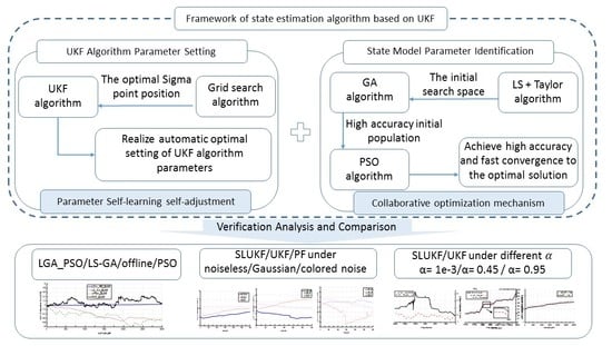
Based on the above two aspects of analysis (state estimator and state model), in order to improve the state estimation accuracy of the model-based UKF estimator, we should start from two aspects: one is to try to achieve the optimal setting of the parameters of the UKF estimator, and the other is to try to improve the accuracy of the state model. So, this paper proposed a combination algorithm. On the one hand, the UKF estimator in the combination algorithm can realize the automatic optimal setting of the parameters in the estimator without human intervention, so that the UKF estimator can run in the optimal situation. The identification algorithm can realize the precise and rapid identification of state model parameters through the cooperation of multiple intelligent parameter algorithms. The improvement of the algorithm from the above two aspects (How to Determine State Estimator Parameters and How to Identify State Model Parameters) can effectively improve the state estimation performance of the UKF algorithm, including accuracy, robustness, etc.

The remaining Sections are organized as follows: In Section 2, the first part of the combination algorithm, that is, the parameter self-learning UKF algorithm, will be introduced in detail. In Section 3, the second part of the combination algorithm, which is a data-driven model parameter identification algorithm, is described. Then, we take the SoC estimation of power battery as the application background and give the overall framework of the combination algorithm proposed in this paper in Section 4. Also taking the SoC estimation as the application background, the verification and comparison of the algorithm will appear in Section 5. Finally, the conclusions for this paper are shown in Section 6.

2. The Parameter Self-Learning Unscented Kalman Filter Algorithm

As mentioned in Reference [10], that when all Sigma points are distributed in an appropriate ellipsoid centered on the mean, the state estimation based on UKF will reach the optimal. In the formula for determining the position of the Sigma points, there are two artificially adjusted parameters: a spread parameter, α, and a scaling factor, κ. Among them, for the state estimation problem, a scaling factor, κ, usually takes zero [11]. Therefore, a spread parameter, α, will become the only artificially set parameter that affects the distribution of Sigma points. Therefore, we hope that the α value can also be adjusted automatically, thereby improving the estimation accuracy of UKF.

First, the general form of the state and measurement Equation of the UKF algorithm is given as follows [12]:

$$\{\begin{array}{c}{x}_t=f(x_{t-1},u_t,w_t)\\ y_t=h(x_t,u_t,v_t)\end{array}$$

(1)

In Equation (1), $x_t$ and $y_t$ represent the state and measured value at time t. $w_t$ and $v_t$ represent the state and measured value noise. The Sigma points of state value are generated by:

$${\tilde{x}}_t\left(i\right)=\{\begin{array}{c}{\overline{x}}_{t-1}^{+},i=0\\ {\overline{x}}_{t-1}^{+}+\sqrt{(n+\lambda )P_{t-1}^{+}},i=1,\cdots ,n\\ {\overline{x}}_{t-1}^{+}-\sqrt{(n+\lambda )P_{t-1}^{+}},i=n+1,\cdots ,2n\end{array}$$

(2)

In Equation (2), $\lambda ={\alpha }^2\left(n+\kappa \right)-n$ is a scale parameter, $\alpha$ represents the divergence of the Sigma points, and $\kappa$ is a scaling factor. Generally, the value of $\kappa$ is zero. n is the dimension of the state variable and $P_{t-1}^{+}$ is the covariance of the state variable.

The state variable weight and covariance weight for each sigma point are given as:

$$W_m\left(i\right)=\{\begin{array}{c}\frac{\lambda }{n+\lambda },i=0\\ \frac{1}{2(n+\lambda )},i\ne 0\end{array}$$

(3)

$$W_c\left(i\right)=\{\begin{array}{c}\frac{\lambda }{n+\lambda }+\left(1-{\alpha }^2+\beta \right),i=0\\ \frac{1}{2(n+\lambda )},i\ne 0\end{array}$$

(4)

In Equations (3) and (4), $W_m(i)$ and $W_c(i)$ are the state variable weight and covariance weight for each sigma point, respectively. $\beta$ is used to represent the prior knowledge of the distribution of the state variable. It is generally considered that the optimal value of $\beta$ is 2.

From the above key steps of the UKF algorithm, it is known that the value of $\alpha$ is extremely important because the value of $\alpha$ determines the position of the sigma points and the calculation result of the two kinds of weights, which affects the execution accuracy of the UKF algorithm [13]. In addition, in the traditional UKF algorithm, the parameter $\alpha$ is not updated after the initial time of the algorithm is set. However, the model parameters have dynamic changes for most systems (such as the power battery system). Therefore, it is reasonable that the selection of $\alpha$ and the location of sigma points should be dynamic and automatic [14,15].

Based on the above requirements, this paper proposes a self-learning mechanism of parameter $\alpha$ based on a grid search algorithm to achieve the purpose of automatically setting and updating key parameter $\alpha$ in the UKF algorithm.

Based on the grid search algorithm, firstly, we take the one-step estimated value of the state variable ${\overline{x}}_{t-1}^{+}(i)$ $i=1,\cdots ,n$ as the center, then a certain range of the high-dimensional space $S_{pace}$ is divided into $Gr\left(i\right)$ $i=1,\cdots ,n$ grid subspaces $S_r\left(i\right) i=1,\cdots ,n$. Gr is the number of grid subspaces. n is the dimension of the state variable. Then, the fitness value $fit(S_r\left(i\right))$ is calculated in each grid subspace $S_r\left(i\right)$ by:

$$fit\left(S_r\left(i\right)\right)=\left|h\left({\tilde{x}}_t{}^{Gr}\left(i\right),u_t,v_t\right)-y_t\right|$$

(5)

In Equation (5), ${\tilde{x}}_t^{Gr}\left(i\right)=x_t^{+}\left(i\right)+k·d_{sr}\left(i\right)$, $i=1,\cdots ,n$, $k=1,\cdots ,Gr\left(i\right)$ is the Sigma point determined by the grid method and $d_{sr}(i)$ represents the width of each subspace $S_r\left(i\right) i=1,\cdots ,n$.

So, the optimal fitness value is:

$$fitbest=\min \left|fit(S_r\left(i\right))\right|$$

(6)

The position determined by the optimal fitness $fitbest$ is the current best position of the sigma points ${\tilde{x}}_t^{Gr\_best}\left(i\right)$. That means:

$${\tilde{x}}_t^{Gr\_best}\left(i\right)=\{\begin{array}{c}{\overline{x}}_{t-1}^{+},i=0\\ {\overline{x}}_{t-1}^{+}+\sqrt{(n+\lambda )P_{t-1}^{+}},i=1,\cdots ,n\\ {\overline{x}}_{t-1}^{+}-\sqrt{(n+\lambda )P_{t-1}^{+}},i=n+1,\cdots ,2n\end{array}$$

(7)

From Equation (7), we can calculate the value of $\lambda$ and $\alpha$:

$$\lambda =\frac{{\left({\tilde{x}}_t^{Gr\_best}\left(i\right)-{\overline{x}}_{t-1}^{+}\right)}^2}{P_{t-1}^{+}}-n$$

(8)

$$\alpha =\sqrt{\frac{\lambda +n}{n+\kappa }}$$

(9)

So far, the parameter self-learning UKF (SLUKF) algorithm proposed in this paper has realized the automatic learning ability of $\alpha$ parameters. Further, according to the $\alpha$ value determined by the grid search algorithm, we can calculate the value of the weights $W_m(i)$ and $W_c(i)$ by Equations (3) and (4).

3. State Model Parameter Identification Algorithm

The intelligent optimization algorithms have a wide range of applications due to their strong global search ability and low mathematical requirements [16]. However, any single optimization algorithm has its own shortcomings in certain environments, such as large computation and slow search speed of GA, partial optimality of the PSO, and weak noise suppression of the LS algorithm. Therefore, an intelligent method based on multi-algorithm collaborative optimization is proposed in this paper for state model parameters’ identification. We use a mechanism of collaborative optimization to unify the LS, GA, and PSO algorithms. The identification method has the advantages of the member algorithms while avoiding the shortcomings of them. It has the high optimization accuracy of the GA algorithm, and uses the LS algorithm to avoid the problem that GA is easily trapped in local optimization. In addition, it has the advantages of fast convergence and low complexity of the PSO algorithm and uses the initialization method based on the GA algorithm to avoid the disadvantage of the low accuracy of the PSO algorithm (We named the identification algorithm proposed in this paper is LGA_PSO algorithm). The general process is as follows:

• Determine the initial search space by the LS algorithm:

Step 1: Nonlinear state model is linearized by first-order Taylor series, which can get a rougher linearization model.

Step 2: We use the LS algorithm to solve the rough linearization model obtained by first-order Taylor series and get the initial solution of state model $P_{ara}$.

Step 3: Then, we use the initial solution $P_{ara}$ as the center of the circle, r as the radius, and n (n is the dimension of the state variable) as the spatial dimension, and determine the hyper sphere to obtain the initial search space of the GA algorithm.

$$ran{g}_{P_{ara}}=\left[min,max\right]=[\left(P_{ara}-r\right)\pm \epsilon ,\left(P_{ara}+r\right)\pm \epsilon ]$$

(10)

where $\epsilon$ is a constant that $\epsilon$→0.

• Get high accuracy initial population of PSO by the GA algorithm

The PSO population initialization flowchart is shown in Figure 1.

In Figure 1, “Parameter initialization” includes the iteration times $mg\_GA$, the cross probability $px$, the mutation probability $pm$ and fitness threshold $fi{t}_{set}$.

“Randomly determine the initial population in the initial search space” uses the Equation (11).

$$P_{ara}{}_{GA}\left(0\right)=Random\left(0,1\right)\times \left(max-min\right)+P_{ara}$$

(11)

“Calculating fitness”: Equation (12) is used to calculate the fitness values.

$$fit\left(g\right)=\left|\widehat{y}\left(g\right)-y\left(g\right)\right|$$

(12)

In Equation (12), $fit\left(g\right)$ and $\widehat{y}\left(g\right)$ are the fitness values and the estimation of measured value, respectively. $g=0,\cdots$ is the number of iterations.

• Get the optimal solution through the PSO algorithm

The flowchart of determining the optimal solution using the PSO algorithm is shown in Figure 2.

In Figure 2, “Parameter initialization” includes the iteration times $mg\_PSO$, the acceleration $c1,$ $c2$ and fitness threshold $fi{t}_{best}$.

“Individual historical optimal solutions and global optimal solutions” includes the best position and fitness value of individual: $p_{best,k}$ and $fi{t}_{best,k}$, $k$ represents the k-th individual, and the global best position and fitness value of the whole swarm: $p_{best}{}^G$ and $fi{t}_{best}{}^G$.

“The Velocity and Position of the Particles Update” uses the following Equations:

$$V_k\left(g^{+}\right)=\omega \times V_k\left(g\right)+c1\times r1\times \left(p_{best,k}-Par{t}_k\left(g\right)\right)+c2\times r2\times (p_{best}{}^G-Par{t}_k\left(g\right))$$

(13)

$$Par{t}_k\left(g^{+}\right)=Par{t}_k\left(g\right)+V_k\left(g^{+}\right)$$

(14)

In Equation (13), $r1$ and $r2$ are the random variables distributed uniformly in the range (0, 1) and $\omega$ is the inertia weight.

4. Application of Combination Algorithm in Battery SoC Estimation

The state of charge of batteries is an important indicator for describing the state of the battery [17,18]. Therefore, online high-precision SoC estimation is critical for battery management systems.

Currently, there are a wide variety of SoC estimation algorithms that have been developed to upgrade the performance of the SoC estimator. Among them, the algorithms that are more suitable for real-time SoC estimation can be roughly divided into: model-based estimation methods [19] and data-driven estimation methods [20]. Model-based estimation methods mainly include AF algorithms (such as EKF and UKF) and observer-based methods (such as sliding mode observer (SMO) and H∞ observer) [21], while data-driven algorithms mainly include Coulomb’s integral algorithm [22], neural network (NN) algorithm [20], and so on. Because completely data-driven SoC estimation methods completely consider the power batteries as a black box, the estimation accuracy depends too much on the training dataset and the quality of the data collected in real time. The observer-based SoC estimation method is prone to the poor tracking performance or the undesired chattering phenomena due to underestimated or overestimated switching gains. In contrast, due to the closed-loop self-correction structure of the AF algorithms taking observation residuals as input, the estimation accuracy of states is high, so AF algorithms have received more attention and have more research results [1].

Based on the above analysis and the detailed introduction of the algorithm in Section 2 and Section 3, we take the SoC estimation of battery as the application background in this part and give the complete framework of the combination algorithm proposed in this paper.

4.1. Power Battery Model

The power battery is a complex system, which is manifested in strong non-linearity. It also has slow time-varying parameters and fast time-varying parameters that change with time. The process data has many transient spikes and contains complex environmental noise. It is almost impossible to establish a simple linear model to characterize its properties. Therefore, the current more common way is to use the equivalent circuit model (ECM) to simulate the complex charging and discharging process of power batteries, such as the Rint model, the N-order RC (Resistor-Capacitance circuit) model ($\mathrm{N}=1,2,\cdots$), the Thevenin model, and the PNGV (The Partnership for a New Generation of Vehicles) model [23]. Except for the Rint model, all are non-linear models. Since the PNGV model is designed for electric vehicles, in this work, we adopted the PNGV model to introduce the model parameter identification algorithm based on the data-driven collaboration mechanism. The PNGV model is shown in Figure 3.

In Figure 3, $U_{ocv}(SoC,T)$ represents the open circuit voltage related with SoC values and temperatures, C_b represents the capacitance of battery, R_e is the internal resistance of battery, R_p is the polarized resistance of battery, C_p is the polarized capacitance of battery, U_d is the terminal voltage of battery, I is the current value of battery, U_b is the voltage of battery across the capacitance C_b, U_p is the voltage of battery across the capacitance C_p, and the battery equivalent model expression is as follows [9]:

$$\{\begin{array}{c}{U}_d=U_{ocv}\left(SoC,T\right)-U_b-U_p-I\times R_e\\ {\dot{U}}_b=\left(1/C_b\right)I\\ {\dot{U}}_p=-\left(1/(C_p{R}_p\right))U_p+\left(1/C_p\right)\times I\end{array}$$

(15)

In Equation (15), ${\dot{U}}_b$ and ${\dot{U}}_p$ are the derivation operation of the voltage Ub and Up, respectively. Then, the discrete model Equation can be obtained from Equation (15) as:

$$\{\begin{array}{c}{U}_{d,t}=U_{ocv}\left(So{C}_t,T_t\right)-U_{b,t}-U_{p,t}-I_t\times R_e\\ U_{b,t}=U_{b,t-1}+\frac{I_t\times \Delta t}{C_b}\\ U_{p,t}=\exp \left(-\frac{\Delta t}{C_p{R}_p}\right)U_{p,t-1}+R_p\times I_t(1-\exp \left(-\frac{\Delta t}{C_p{R}_p}\right))\end{array}$$

(16)

In Equation (16), $U_{d,t}$ represents the terminal voltage at time t, $U_{ocv}(So{C}_t,T_t)$ represents the open circuit voltage related with $SoC$ values and temperatures at time t, $U_{b,t}$ and $U_{p,t}$ represent the terminal voltages across $C_b$ and $C_p$ at time t, Δt represents the sample period, and $I_t$ represents the current value at time t.

Based on Equation (16), the parameter vector $\gamma$ can be obtained. The expression is as follows:

$$\gamma ={\left[\begin{array}{c}{C}_b\\ R_p\\ C_p\\ R_e\end{array}\right]}^T$$

(17)

4.2. Application of Combination Algorithm in Battery SoC Estimation

Based on the PNGV model of Equation (16) and the Coulomb integral SoC calculation method, the state Equation of the power battery is obtained as follows [24]:

$$\begin{gathered} So{C}_t=So{C}_{t-1}+\frac{\eta \left(T_t,I_t\right)·\Delta t}{C_n}·I_t \\ {U}_{d,t}=U_{ocv}\left(So{C}_t,T_t\right)-U_{b,t-1}+\frac{I_t\times \Delta t}{C_b}-\exp \left(-\frac{\Delta t}{C_p{R}_p}\right)U_{p,t-1}+R_p\times I_t\left(1-\exp \left(-\frac{\Delta t}{C_p{R}_p}\right)\right)-I_t\times R_e \end{gathered}$$

(18)

In Equation (18), $t$ represents the sample moment, $\eta \left(T_t,I_t\right)$ represents the battery capacity factor related with $T_t$ and $I_t$, and $C_n$ represents the rated capacity.

According to Equation (18) and the novel combination framework proposed in this paper, we can build a flowchart of SoC estimation, which is shown in Figure 4.

A: “Get initial $SoC$ by Open Circuit Voltage Method” in the initialization part of flowchart: This step is only used once at the initial moment when the electric vehicle battery management system (BMS) is powered on. At this time, since the power battery has been left standing for a long enough time, we think the Equation $U_{d,}\left(0\right)=U_{ocv}$ holds.

B: In Equation (18), the open-circuit voltage value $U_{ocv}(So{C}_t,T_t)$ at different $SoC$ and temperatures is obtained according to the data of the power battery manual and laboratory measurement data. During the operation of the algorithm proposed in this paper, $U_{ocv}(So{C}_t,T_t)$ is obtained by looking up the table through different $SoC$ values and temperatures.

5. Algorithm Verification Analysis and Comparison

Here, we take the battery SoC estimation as the application background and compare it with traditional methods to verify the advantages of the proposed algorithm in terms of accuracy, robustness, and complexity. Algorithm verification and comparison are from the following aspects:

• LGA_PSO algorithm accuracy verification and comparison: To achieve SoC estimation, the LGA_PSO algorithm, LS_GA algorithm (The combination method by LS and GA), offline identification algorithm, and PSO algorithm are combined with the SLUKF estimation method proposed in this paper, separately. By comparing the SoC estimation results, the accuracy advantage of the LGA_PSO algorithm proposed in this paper is verified from the side.
• SLUKF algorithm accuracy verification and comparison: The LGA_PSO algorithm is combined with the SLUKF algorithm, the UKF algorithm, and the PF algorithm respectively, to realize the SoC estimation, and the accuracy of the SLUKF algorithm proposed in this paper is verified by comparing the SoC estimation results.
• In order to verify the robustness advantages of the SLUKF algorithm proposed in this paper, the estimated performance of the UKF algorithm is compared with the SLUKF algorithm under different $\alpha$ conditions.
• The complexity of the LGA_PSO_SLUKF algorithm (The combination of the SoC estimation method proposed in this paper. That is LGA_PSO and SLUKF), GA_SLUKF algorithm (The combination method by GA and SLUKF), and GA_UKF algorithm (The combination method by GA and UKF) are compared to verify the complexity advantage of the LGA_PSO_SLUKF algorithm proposed in this paper.
• The SoC estimation is performed under no-noise, Gaussian noise, and colored noise conditions to verify the robustness of the LGA_PSO_UKF (The combination method by LGA_PSO and UKF) algorithm.

5.1. Test Platform and Data Introduction

The experimental verification is divided into two parts:

• The first part: “the verification of the model parameter identification accuracy based on the LGA_PSO algorithm by hardware-in-the-loop equipment [25]”.
  In this paper, we use a LG 18,650 battery parameter (shown in

  Table 1. The LG 18,650 battery detailed information.

  Capacity	Nominal Voltage	Max Voltage	Min Voltage
  36 Ah	3.6 V	4.15 V	2.5 V

  ) to set the battery model in the HIL (Hardware-in-the-Loop and is shown in Figure 5a), and use this battery model to simulate the characteristics of the actual battery during charge and discharge in this verification process. For the power battery model in this HIL, we take the actual NEDC (New European Driving Cycle) operating condition discharge current (shown in Figure 5c) as the model input, measure the output of the power battery model, and compare it with the LGA_PSO identification results proposed in this paper.
• The second part: “The verification and comparison of the parameter SLUKF algorithm effectiveness by a test platform with battery charging and discharging equipment (shown in Figure 5b)”.
  During this verification process, we use a real LG18650 battery to perform tests to make it discharge according to the discharge current of the actual NEDC operating conditions (shown in Figure 5c), and collect its measured $SoC$ value (shown in Figure 5f) and terminal voltage (shown in Figure 5c) as the true value to analyze and compare the performance of the parameters of the self-learning UKF algorithm proposed in this article. Also, in this part of the verification process, in order to be more realistic and close to the actual situation, we add Gaussian white noise and colored noise signals to the current under NEDC operating conditions and the collected terminal voltage to generate noise-containing current and voltage signals (shown in Figure 5d,e).

5.2. LGA_PSO Model Identification Algorithm Accuracy Verification and Comparison

In this part, the parameters’ determination capability of the LGA_PSO algorithm is analyzed. We used the LGA_PSO algorithm to identify the parameter $\gamma$ of ECM in Equation (12) within the SoC range [0.3, 0.9], and based on the identification results, the total internal impedance value of the ECM Resti is calculated. Then, Resti is compared with the parameter values measured from the battery model, the results are shown in

Table 2. Parameter Identification Results.

SoC (%)	Uocv/V	$\mathit{Resti}/\mathit{m}\mathbf{\Omega }$	$\mathit{Rober}/\mathit{m}\mathbf{\Omega }$
30	3.5941	2.77	2.75
40	3.6242	1.78	1.79
50	3.6603	1.59	1.63
60	3.7302	1.65	1.62
70	3.8350	1.61	1.65
80	3.9260	1.66	1.68
90	4.0259	1.64	1.69

.

In Table 2, Uocv is measured open circuit voltage of the battery. Resti represents the total internal impedance value of the ECM calculated by the LGA_PSO algorithm and Rober represents the total internal impedance value from the battery model. The result shows that the MaxE (Maximum Error) of the total internal impedance is 0.02 mΩ, the error is less than 1%. It shows that the LGA_PSO algorithm proposed in this paper has excellent accuracy in model identification.

Furthermore, we combine the LGA_PSO-based parameter identification algorithm proposed in this paper, the traditional PSO parameter identification algorithm, the LS_GA parameter identification algorithm, and an offline algorithm (only using the parameter values given in the LG manual) with the SLUKF algorithm, respectively. Then, through comparing accuracy of estimating SoC by different combination algorithms to compare the performance of different model parameter identification algorithms, the verification results are shown in Figure 6.

According to Figure 6a, the comparison results of SoC by the different parameter identification methods combined with the SLUKF estimator can be known, and the SoC estimation error of different methods is shown in Figure 6b. It can be found that the SoC estimation error of the LGA_PSO_SLUKF algorithm is less than 1% while the SoC estimation error of the offline_SLUKF (The combination method by offline algorithm and SLUKF) method, the LS_ GA_SLUKF (The combination method by LS_GA and SLUKF) algorithm, and the PSO_SLUKF (The combination method by PSO and SLUKF) algorithm are about 5%, 2%, and 2.2%. The comparison results demonstrate that the LGA_PSO_SLUKF algorithm can enhance the accuracy of the SoC estimation. This also reflects that the proposed LGA_PSO collaborative optimization mechanism method has higher model parameter identification accuracy than the traditional LS_GA algorithm and PSO algorithm. The reason for this is that although PSO has a fast convergence speed, the accuracy is low, the GA algorithm converges so slowly that it is difficult to achieve the desired accuracy in a limited calculation period, and the LS algorithm has poor accuracy in nonlinear systems. Therefore, the performance of the above algorithms when used alone is worse than that of a combination algorithm with a cooperative mechanism. In addition, due to the problem of battery consistency, the offline parameters of the battery cannot reflect the true battery performance anymore, so that the accuracy of the SoC estimation based on this is not satisfactory.

Finally, the SoC estimation is performed by repeatedly using the LGA_PSO algorithm, LS_GA algorithm, PSO algorithm, and the offline method in combination with the SLUKF algorithm. The error comparison results are shown in

Table 3. Error stability comparison results.

Algorithm	Operation Times	MaxE (%)	RMSE (%)
Offline_SLUKF	70	[2.7887, 4.2642]	[1.7424, 2.9302]
LS_GA_SLUKF	70	[2.1561, 3.8450]	[1.1006, 2.5701]
PSO_SLUKF	70	[0.9269, 6.0511]	[0.5214, 3.1489]
LGA_PSO_SLUKF	70	[0.3215, 0.7260]	[0.1586, 0.2687]

.

In Table 3, MaxE is maximum error, and RMSE is root mean square error. And Table 3 shows the error results of the LGA_PSO_SLUKF method and other traditional methods after repeated operations. The results show that the LGA_PSO_SLUKF algorithm with MaxE less than 1% and RMSE less than 0.3% has better accuracy in model recognition than the usual offline _SLUKF method, LS_GA_SLUKF algorithm, and PSO_SLUKF algorithm.

5.3. SLUKF State Estimation Algorithm Accuracy Verification and Comparison

In order to compare and verify the accuracy advantages of the SLUKF-based SoC estimation method, we used the second part of the test platform introduced in Section 5.1. The comparison verification process is divided into three cases: a noiseless environment, a white noise environment, and a colored noise environment [26]. In the above three noise situations, we used the LGA_PSO_SLUKF algorithm, the LGA_PSO_UKF algorithm, and the LGA_PSO_PF algorithm (The combination method by LGA_PSO and PF) to perform SoC estimation to compare the performance of each state estimation method in estimation accuracy under the same model accuracy.

Table 4. Initial Parameters of SLUKF Algorithm.

${\mathit{\alpha }}_0$	$\mathit{\beta }$	$\mathit{\kappa }$	$\mathit{p}\mathit{o}\mathit{p}\mathit{s}\mathit{i}\mathit{z}\mathit{e}$	$\mathit{p}\mathit{x}$	$\mathit{p}\mathit{m}$	$\mathit{\omega }$
${10}^{-3}$	2	0	16	0.8	0.01	0.7928

lists the initial parameters of the LGA_PSO_SLUKF algorithm.

1. Case 01: SoC estimation under noiseless condition: Firstly, the performance of the LGA_PSO_SLUKF algorithm, LGA_PSO_UKF algorithm, and LGA_PSO_PF algorithm are compared under noise-free conditions.

Figure 7 shows that the MaxE of the LGA_PSO_SLUKF estimator is less than 0.4%. The MaxE of the LGA_PSO_UKF-based SoC estimate and the LGA_PSO_PF-based SoC estimate are about 0.5% and 0.6%, respectively. From the perspective of accuracy, in a noise-free environment, the performance of the three state estimation methods is equivalent, and the accuracy of the SLUKF algorithm proposed in this paper is slightly better. The reason is that in a noise-free environment, the system has fewer disturbances. When the traditional UKF parameter $\alpha$ is selected reasonably, it also has better accuracy. However, there is a stable error in the PF algorithm estimation.

2. Case 02: SoC estimation under the Gaussian noise condition. Secondly, under the condition of Gaussian noise, we compared the performance of the LGA_PSO_SLUKF algorithm, the LGA_PSO_UKF algorithm, and the LGA_PSO_PF algorithm.

The estimation results are shown in Figure 8. It can be expected that we can find that the MaxE of the LGA_PSO_SLUKF SoC estimator is about 0.5%. However, the maximum MaxE of the LGA_PSO_UKF SoC estimator and the maximum error of the LGA_PSO_PF SoC estimator are approximately 1.1% and 0.8%, respectively. This is because it is difficult for the traditional UKF to give the optimal position of the Sigma points when the system is disturbed, while the SLUKF algorithm can still achieve the optimal position of the Sigma points by optimization. Therefore, even in a noisy environment, the SLUKF algorithm still has good accuracy. In addition, because the number of particles in the PF algorithm is larger than the number of Sigma points in the traditional UKF algorithm, the tracking state variance is better, so its accuracy is relatively high. But, this accuracy comes at the expense of computational complexity.

3. Case 03: SoC estimation under the colored noise condition. In this case, the performance of the LGA_PSO_SLUKF method, LGA_PSO_UKF algorithm, and LGA_PSO_PF algorithm under colored noise conditions will be compared, respectively. Colored noise is added to the current and terminal voltage. And the comparison results are shown in Figure 9.

According to the above comparison process, it can be concluded that because the SLUKF algorithm proposed in this paper can optimize the position of the Sigma point, it has better anti-interference performance. The performance is significantly better than the traditional UKF algorithm in a noisy environment. Because the traditional PF algorithm has a large number of particles, the ability to track statistics such as state variance is better than UKF. Therefore, its performance is better than the UKF algorithm in a noisy environment, and even comparable to the SLUKF proposed in this paper. But, this comes at the expense of computational complexity, which will be explained in a later section.

5.4. Comparison of SLUKF Convergence under Different α Values

By comparing the estimated performance of the SLUKF algorithm and the traditional UKF algorithm at different α values, the robustness of the proposed SLUKF algorithm and the self-adjusting effectiveness of the scale parameter α are verified. We set different α values for the SLUKF algorithm and the UKF algorithm, and then compared the performance of the SLUKF algorithm and the traditional UKF algorithm. The comparison results are shown in Figure 10.

The comparison results show that the traditional UKF and SLUKF have similar estimation accuracy when the α parameter value is appropriate (α = 1e − 3), but when the α parameter manually set by the traditional UKF algorithm is incorrect (α = 0.45 or 0.95), its accuracy is obviously worsened, or it no longer converges (α = 0.95), while the SLUKF algorithm proposed in this paper can obtain the appropriate value through its own optimization when the initial α parameter setting is incorrect, thereby ensuring the estimation accuracy of the algorithm. Therefore, it has strong robustness and is suitable for SoC estimation under different working environments.

5.5. Verification and Comparison of Computational Complexity of LGA_PSO_LSUKF Algorithm

Here, the complexity of the GA_SLUKF algorithm is compared with the GA_PF (The combination method by GA and PF) algorithm to verify the advantages of the SLUKF algorithm in computing complexity. At the same time, the complexity of the GA_SLUKF algorithm and the LGA_PSO_SLUKF algorithm are compared to verify the advantages of the LGA_PSO collaborative optimization algorithm proposed in this paper in terms of computational complexity. The comparison results are shown in

Table 5. Time complexity of SoC estimation comparison results.

SoC Estimation Algorithm	Operation Times	One Iteration	Total Time
GA_SLUKF	70	32.1 ms	96.3 s
GA_PF	70	38.6 ms	115.8 s
LGA_PSO_SLUKF	70	30.4 ms	91.2 s

.

According to Table 5, it can be seen that one operation time of the LGA_PSO_SLUKF method is 30.4 ms, and the total time is 91.2 s. One iteration time of the GA_SLUKF algorithm is 32.1 ms, and the total operation time is 96.3 s. The GA_PF algorithm has an iteration time of 38.6 ms and a total operation time of 115.8 s. This shows that the convergence speed of the LGA_PSO algorithm proposed in this paper is significantly better than that of the traditional GA algorithm, while the SLUKF algorithm proposed in this paper is equivalent to the traditional PF algorithm in accuracy, but it is significantly better than the traditional PF algorithm in calculation time.

5.6. Comparison of Stability of LGA_PSO_SLUKF Algorithm under Noise Conditions

We know that the stability of the optimization algorithms is relatively weak. The SoC estimator has very high requirements for the stability of the algorithm. Therefore, the stability of the proposed LGA_PSO_SLUKF algorithm under different noise environments is validated. The validation results are plotted in

Table 6. Stability verification results of LGA_PSO_SLUKF algorithms.

Noise	Operation Times	MaxE (%)	RMSE (%)
Noiseless	70	[0.3215, 0.7260]	[0.1586, 0.2687]
Gaussian Noise	70	[0.4340, 0.8036]	[0.2457, 0.4253]
Colored Noise	70	[0.7177, 1.1729]	[0.5311, 0.6998]

.

Based on verification results, we can conclude that the MaxE of the LGA_PSO_SLUKF SoC estimator is less than 1.2%, and the RMSE is less than 0.7%. It indicates that the stability of the LGA_PSO_SLUKF algorithm under noise condition is also better, which can meet the engineering requirements.

6. Conclusions

In this paper, we proposed a combined architecture of adaptive filtering. The core innovation of the architecture is as follows: First, a novel parametric self-learning UKF (SLUKF) algorithm was proposed in this paper. By optimizing the position of the Sigma points, dynamic self-learning and self-adjustment of α parameters and weights in the UKF algorithm are achieved, thereby improving the accuracy of the state estimation of the UKF algorithm. At the same time, for non-linear system models, such as battery model equivalent circuit models, a collaborative optimization mechanism (LGA_PSO) method was proposed to track the parameters’ change of the identification model. This mechanism can well describe the dynamic characteristics of the state model, and quickly and accurately calculate the model parameters in real time. Finally, this paper applied the proposed combined architecture to the SoC estimation of power batteries, achieving better estimation accuracy and robustness.

In the verification part, we verified the accuracy, noise immunity, robustness, computational complexity, and stability of the LGA_PSO and SLUKF algorithms proposed in this paper by comparing with traditional algorithms. Experimental results showed that compared with the LS_GA algorithm and the PSO algorithm, the proposed LGA_PSO algorithm has higher accuracy and better stability. Compared with the traditional UKF algorithm, the SLUKF algorithm has stronger anti-noise and robustness because it can automatically optimize the position of Sigma points. Compared with the traditional PF algorithm, the SLUKF algorithm has the same calculation accuracy and lower calculation complexity.