Novel Twofold Use of Photographic Technique for Simultaneous Flow Boiling Image Recording and Void Fraction Computation in a Mini-Channel Experiment

Abstract

The paper presents a novel twofold use of the photographic technique for flow boiling heat transfer investigation in the horizontal mini-channel. The dedicated measurement system was constructed to record basic thermal and flow parameters, i.e., boiling liquid inlet and outlet temperatures and pressures, and also temperatures inside the heating block to calculate heat flux going into the liquid. A high-speed video camera equipped with synchronous movement system was applied to combine the recording of two-phase flow images with simultaneous local void fraction measurements both based on the same photographic data set. The data were collected, managed, and refined with the scripts developed in the MathWorks Matlab 2019b environment. The synchronous use of two intelligent techniques in the scripts, i.e., the background subtraction technique and the statistical analysis of individual pictures allowed obtaining reliable experimental results. The proposed method of the void fraction determination ensures high measurement accuracy.

1. Introduction

High heat flux dissipation is a serious challenge faced by a number of industries. Electronic integrated circuits, processors, graphical modules, and power supply modules produce large amounts of heat and require intensive cooling. Heat fluxes generated by these devices are extremely high and can reach up to 1 MW/m².

Phase change in boiling can be used to obtain high heat fluxes at small temperature differences between the heat emitting surface and cooling liquid and at small dimensions of the heat transfer system as well. Heat transfer to a boiling liquid flowing in mini-channels is a modern way of heat transfer enhancement in small, mostly electronic devices. Visualization and quantification of boiling is important not only for its application on a small scale but also for its understanding and modeling in the macro scale. The microscale results can be applied to verify numerical models of boiling heat transfer for industrial needs.

To investigate heat transfer and vapor generation in flow boiling, various physical parameters must be determined at different levels of measurement difficulty. The values of the local void fraction, that is, the fraction of the channel volume occupied by the vapor phase at a given cross-section of the channel measured in parallel with two-phase flow pattern recognition are the most demanded data for theoretical modeling and numerical calculations. Combining the recording of two-phase flow images with simultaneous local void fraction measurements both based on the same photographic data set and using intelligent data processing was the aim of the research presented here.

2. Analysis of Experimental Methods for Void Fraction Measurement

Various experimental methods have been applied to measure local, mean, or instantaneous void fraction in the mini-channel under two-phase flow conditions (liquid and gas or liquid and its vapor). The most frequently used methods are briefly presented and the examples of the most recent works in the field are given.

The quick-closing valve method (QCV) is a very important, simple, and effective method used to measure the mean value of void fraction in the channel. After the simultaneous closure of two valves located at the channel inlet and outlet, the liquid gathers in the lower part of the channel and gas or vapor in the upper one. This allows determining the position of the interface and calculating the volume fractions of both phases. Srisomba et al. [1] applied this method to measure the vapor void fraction of R-134a flowing in a horizontal tube. The void fraction increased with the growing saturation temperature, but the mass flux did not have any important impact on its value [1]. Wongwises and Pipathattakul [2] applied the quick-closing valve method in measuring void fraction in two-phase flow of liquid and gas in the inclined annular channel, and Xue et al. [3] used it in the study of two-phase downward flow in vertical tubes. In two cases [2,3], the authors demonstrated an important impact of the channel inclination on the measured void fraction and pressure drop. They also found the quick-closing method unsuitable for measuring local and instantaneous void fractions.

The methods based on radiation attenuation phenomenon of X, β, and γ-rays allow measuring the instantaneous and local values of the void fraction without disturbing the flow. The most frequently used is the γ-ray technique because radioactive isotopes can be used as a radiation source. The much smaller range of β-rays and costly and complicated design of X-ray sources limits their application in two-phase flow experiments. Waelchli et al. [4] applied tomographic Roentgen transmission microscopy (XTM) for the visualization of water–air two-phase flow in microchannels, and Nazemi et al. [5] determined void fractions in two-phase flow of engine oil and air by measuring γ-ray attenuation. High accuracy of the experimental results was declared in both cases. This accuracy deteriorated substantially with decreasing differences between the gas and liquid radiation absorption.

Different electrical and optical resistances of gas and liquid were used in resistance probes to measure void fraction and length of gas or liquid plugs in adiabatic two-phase flow of nitrogen and water [6]. The probes were made of fast-responding optical fibers and infrared photodiodes, which allowed measurement of local or mean void fraction depending on their mutual location along the microchannel. For artificially generated and stable two-phase flow, the resistance probe method guaranteed high accuracy but the obtained results and the authors raise doubts if the method could be adequate under dynamic flow boiling conditions [6].

Recently, the electrical capacitance method has gained attention of many researchers. This method is limited to electrically non-conductive fluids. It is based on the differences of electrical constants of two phases present in the flow. The capacity measured between one or more pairs of electrodes mounted on the opposite sides of the channel depends on the volume ratios of the two phases. The capacitor has the largest capacity for the channel fully filled with liquid and its value goes down when the void fraction increases. This measurement method does not allow synchronous observation of two-phase flow structures because the observed volume of the channel is shielded by the electrodes. Many examples of effective application of the capacitance method can be found in the works of Roman et al. [7]—measurements of void fraction in R134 flow through 7 mm tube; Caniere et al. [8]—analysis of horizontal two-phase flow in small diameter tubes; He et al. [9]—development of multi-wire capacitance probe; and Maeno et al. [10]—void fraction measurements in two-phase cryogenic flow. De Kerpel et al. [11] proposed the utilization of specific features of capacitance signal for its calibration and measuring void fraction in small diameter tubes. Rocha et al. [12,13] designed a dedicated capacitance sensor to measure void fraction in the refrigeration cycle, which proved its efficiency in investigating two-phase flow in the pilot refrigeration installation. The authors declare high accuracy of the measurements but emphasize that the results depend on the two-phase flow configuration and electrode angle dimensions.

The substantial difference in acoustic velocity between gas and liquid has been used in the acoustic method of void fraction measurement. Al-lababidi et al. [14] applied this method to measure void fraction in gas–liquid slug flow and proposed their correlation for the void fraction calculation. To determine void fraction, Cavaro [15] used the results of low frequency acoustic velocity measurements in air microbubble clouds generated in water. The measurements covered quite a narrow range of void fraction in a flow without boiling. In the literature dealing with boiling, the examples of acoustic method application can hardly be found.

Gui et al. [16] measured local and average void fractions for vapor and water mixture in a rod bundle geometry by three various methods: the optical probe, γ-ray densitometry, and differential pressure method. Compatibility of the experimental results coming from all the methods was at the level of ±15%.

None of the discussed void fraction experimental methods appeared suitable for synchronous measurement of void fraction and two-phase flow boiling structure. The main weaknesses of all methods were as follows:

-

Quick closing valve method (QCV) is inappropriate by its design to measure local void fraction and record local two-phase flow boiling structure;

-

The accuracy of the methods based on radiation attenuation of X, β, and γ-rays deteriorates substantially with decreasing differences between the gas and liquid absorption; for synchronous recording of two-phase flow structures, additional video equipment is required;

-

The accuracy of various electrical and optical resistance probes has not been verified in dynamic flow boiling conditions; for synchronous recording two-phase flow structures, additional video equipment is required;

-

The electrical capacitance method does not permit synchronous observation of two-phase flow structure because the observed volume of the channel is covered by the electrodes.

The only way to get reliable information about instantaneous local void fraction and images of corresponding local two-phase flow structure in dynamic boiling conditions appears to be the intelligent application of the photographic method. By using this method, it is possible to record two-phase flow structure images, with controlled accuracy and controlled high speed, appropriate for the dynamics of the observed process.

3. Digital Image Processing Method

The goal of this research is to obtain data from the same source to record the image of two-phase flow and measure the corresponding void fraction. The most suitable method meeting this condition is the digital image processing method (DIP), which requires transparent channel walls for taking and processing photos (video frames). A detailed analysis of the obtained image allows the determination of local and instantaneous value of void fraction and description of the corresponding two-phase structure. With this method the development of flow boiling can be observed from its incipience to the full evaporation of the liquid.

Until now, fast film cameras have not been used for determining void fraction alone. The two-phase flow structures were recorded in combination with another method that measured void fraction. For instance, Roman et al. [7] and Caniere et al. [8] combined the camera recording of two-phase flow structures with different electrical capacitance methods for two-phase flows in small diameter tubes.

Processing the video frames (or photographs) involves two sources of information that can be used to detect and follow the objects of interest. These are visual features like color and shape, and the features of the object’s motion. Two different techniques are required to process and combine the information from both sources.

The background subtraction technique is commonly used in motion segmentation [17,18]. The outcome of pixel subtraction from the image containing a moving object of interest is the image of that object. Morphological processing operations that follow are: erosion, expanding and closing, and final filtration for noise removal and better recognition of the tracked objects. The background subtraction technique efficiently detects the majority of important pixels of the moving objects regardless of their velocity. However, this technique is sensitive to all kinds of dynamic changes during image processing. For instance, uneven illumination may generate shadows incorrectly read as pixels of the tracked object.

The second technique applied in image processing is the statistical analysis of individual pixels [17,18,19]. It was developed to overcome difficulties encountered in background subtraction techniques. The statistical approach is used for updating the current data of colors in each pixel. Identification of pixels of the foreground, which are the moving objects, is based on the comparison of their colors with the colors of the background. The new moving objects detected in the observed region require more operations (more time) to be qualified as a part of the background than the pixels already included in it. During data collection over time, operation after operation, the statistical evaluation whether a certain pixel can be classified as a background or belongs to the tracked object is possible because the statistical color map representing object’s pixels is built, which is wider than the statistical background color map. Finally, thanks to the comparison of both maps, object detection is possible. This technique proved to be effective for images affected by noise, non-uniform lighting, and shadows.

Combined application of both presented techniques allow the elimination of the majority of errors of dynamic detecting and tracking vapor bubbles in two-phase boiling flow. Both were used to process images of two-phase boiling flow structures in the mini- channel, obtained with a high-speed video camera. The same images were taken for flow structure description and void fraction calculation. Two Matlab software packages, Computer Vision and Image Processing Toolbox were used in our scripts designed for performing image processing, namely, the background subtraction and the statistical analysis of individual pictures to get the data resulting from this experiment [18].

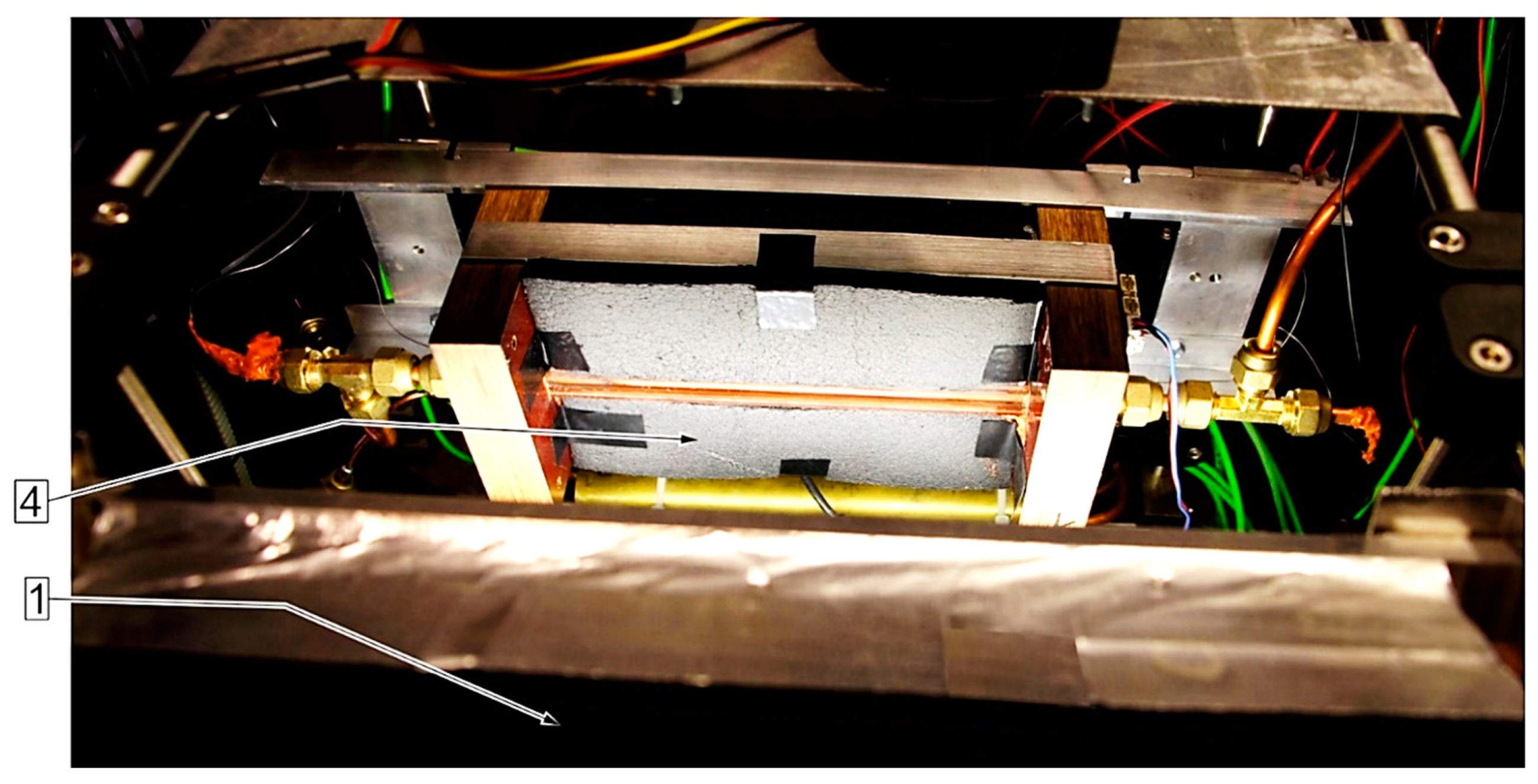
4. Experimental Stand

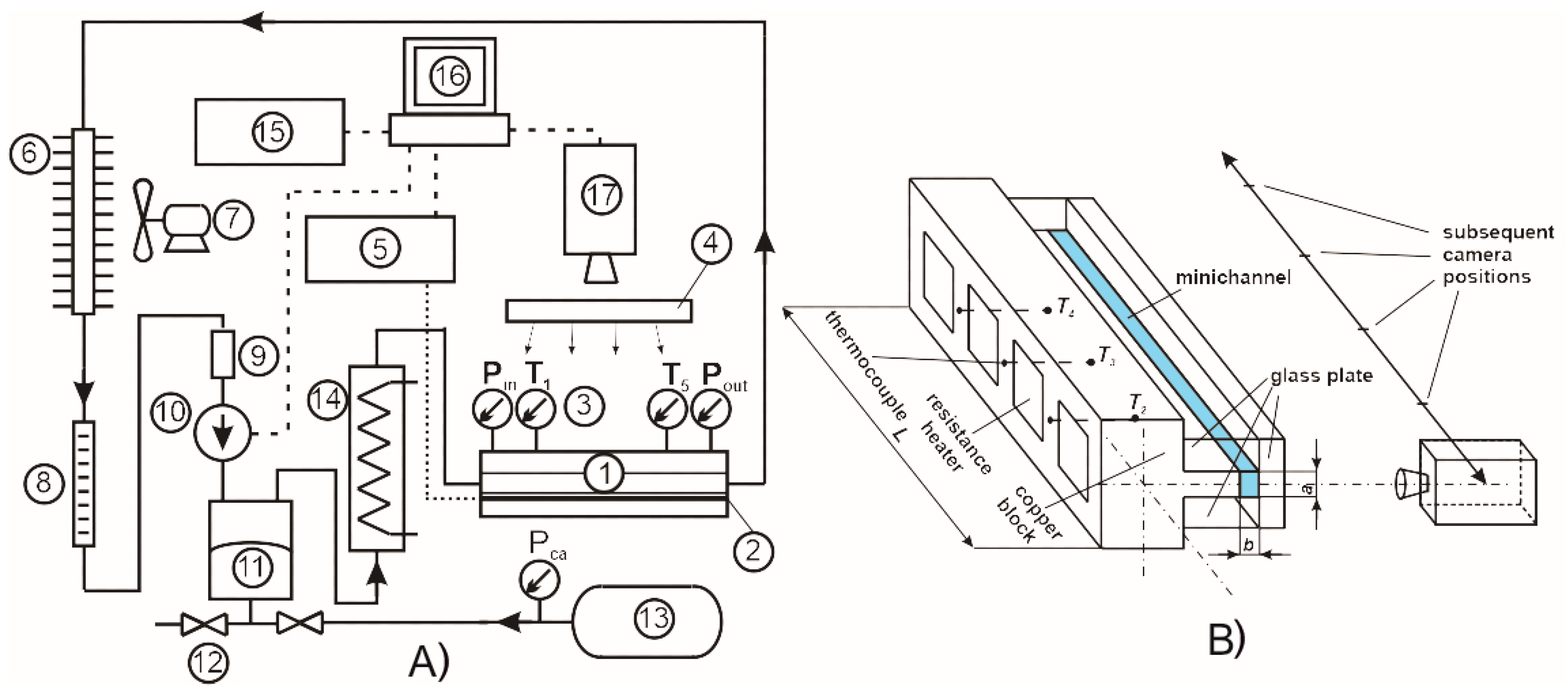
The basic element of the experimental stand, Figure 1A, was the measurement module, Figure 1B, with the horizontal mini-channel to observe from three sides two-phase flow structures formed during the experimental run.

Figure 1a shows the diagram of the flow loop. The heated fluid—in this case, water—leaves the channel (1) towards the cooler (5) and is directed through the rotameter (7), filter (8), and precision micropump (9) to the pressure control device (10) with elastic rubber diaphragm. The compressed air pressure (12) determines the pressure in the flow system. From the pressure control device, the fluid flows to the pre-heater (13) and finally to the mini-channel (1). Heating of the mini-channel, Figure 1B, is done by four heating resistors powered by direct current power supply. The resistors are located on the opposite side of the copper block. Three thermocouples installed in the body of the copper block measure its temperature. Temperatures and pressure at the mini-channel inlet and outlet are also recorded (3).

The mini-channel, Figure 1B, is 180 mm long—L, 1.5 mm deep—b, and 4 mm wide—a, which gives the rectangular cross section of 6 mm² and a hydraulic diameter of 2.18 mm. Three walls of the mini-channel are made of Optiwhite glass tiles, while the fourth one is the heater milled from a copper block. Optiwhite is colorless, super transparent float glass containing very limited amount of iron and having the highest light-transmission coefficients. Three transparent walls of the channel enable proper lighting and recording the boiling two-phase structures with a high-speed camera.

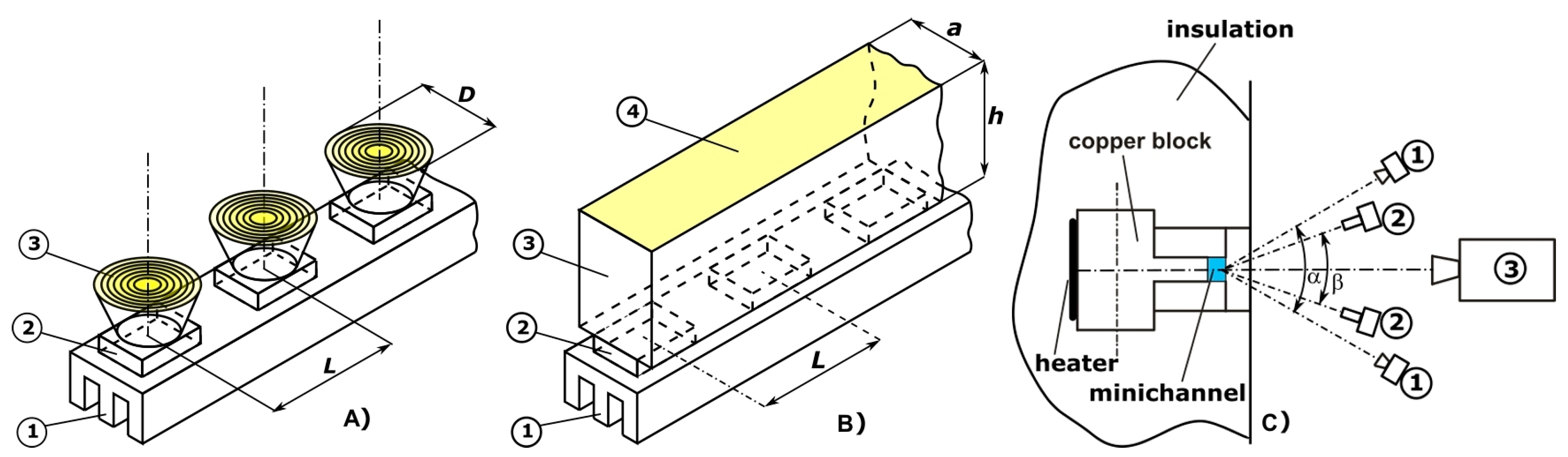
For two-phase flow images to be properly recorded with high speed (up to 7000 frames per second), the camera requires very intensive lighting. An LED lighting system of the authors’ own design, Figure 2, was implemented to avoid the mini-channel heating by high-output incandescent light, which could lead to an additional measurement error. Moreover, the light source should not generate any shadows or reflections. As a result of many experiments, the LED lighting system was chosen with two different types of illuminators: type (A)—generating the diffused light, and type (B)—generating the focused light. Type (A) was composed of Fresnel lenses, Figure 2A, and type (B) was light transmitting plexiglass layer, Figure 2B. Both illuminators had a shape of longitudinal rails, 280 mm long, composed of aluminum radiator, LED illuminators, and elements shaping the light beam (Fresnel lenses or plexiglass layer). Spatial mutual location of the illuminators for the camera was a very important factor in ensuring the required lighting inside the mini-channel. The best results were obtained experimentally for symmetric locations of illuminators towards the camera and for two different angles of optic axes intersections, α = 60 and β = 20, Figure 2C.

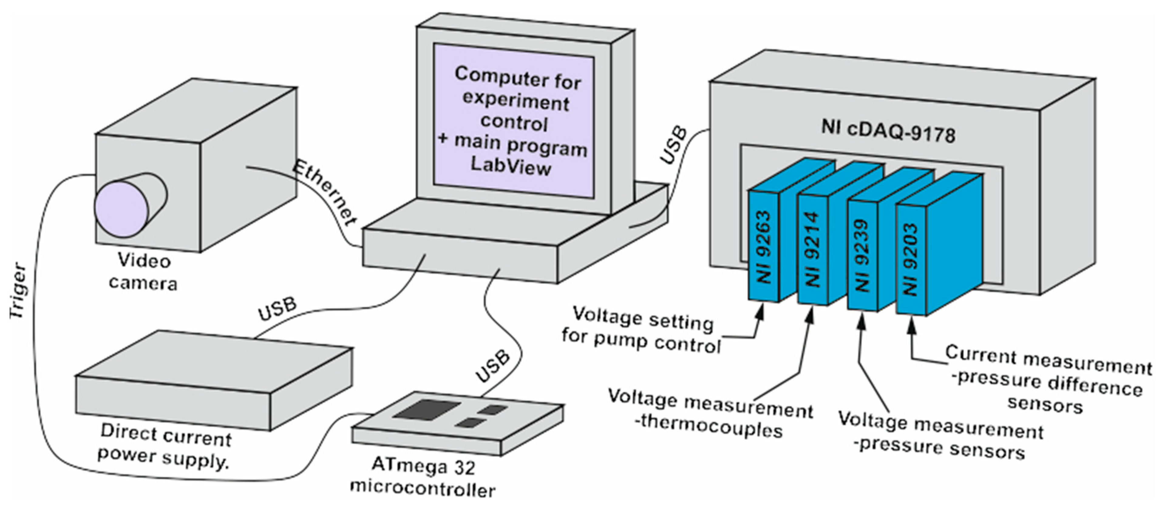
The data acquisition and control system based on the LabView program and National Instruments modular hardware managed the operation of the stand components and the reading and recording the experimental data, Figure 3. LabView was chosen due to its versatility and support to the control-measurement modules. The main module NI cDAQ-9178 controlled the cooperating measurement modules: NI 9214—temperature (thermocouples); NI 9239—pressure (Kobold sensors); and NI 9203—pressure drop (KOBOLD sensor) and NI 9263—flow rate (the gear pump).

During the experimental run, a huge amount of data of various types had to be recorded. To speed up the overloaded acquisition system, an additional control module based on ATMega 32 [Microchip, Chandler, Arizona, USA] microcontroller was designed and implemented. The program written in the BASCOM [MCS Electronics, Almere, Holland] environment was used to control the high-speed camera.

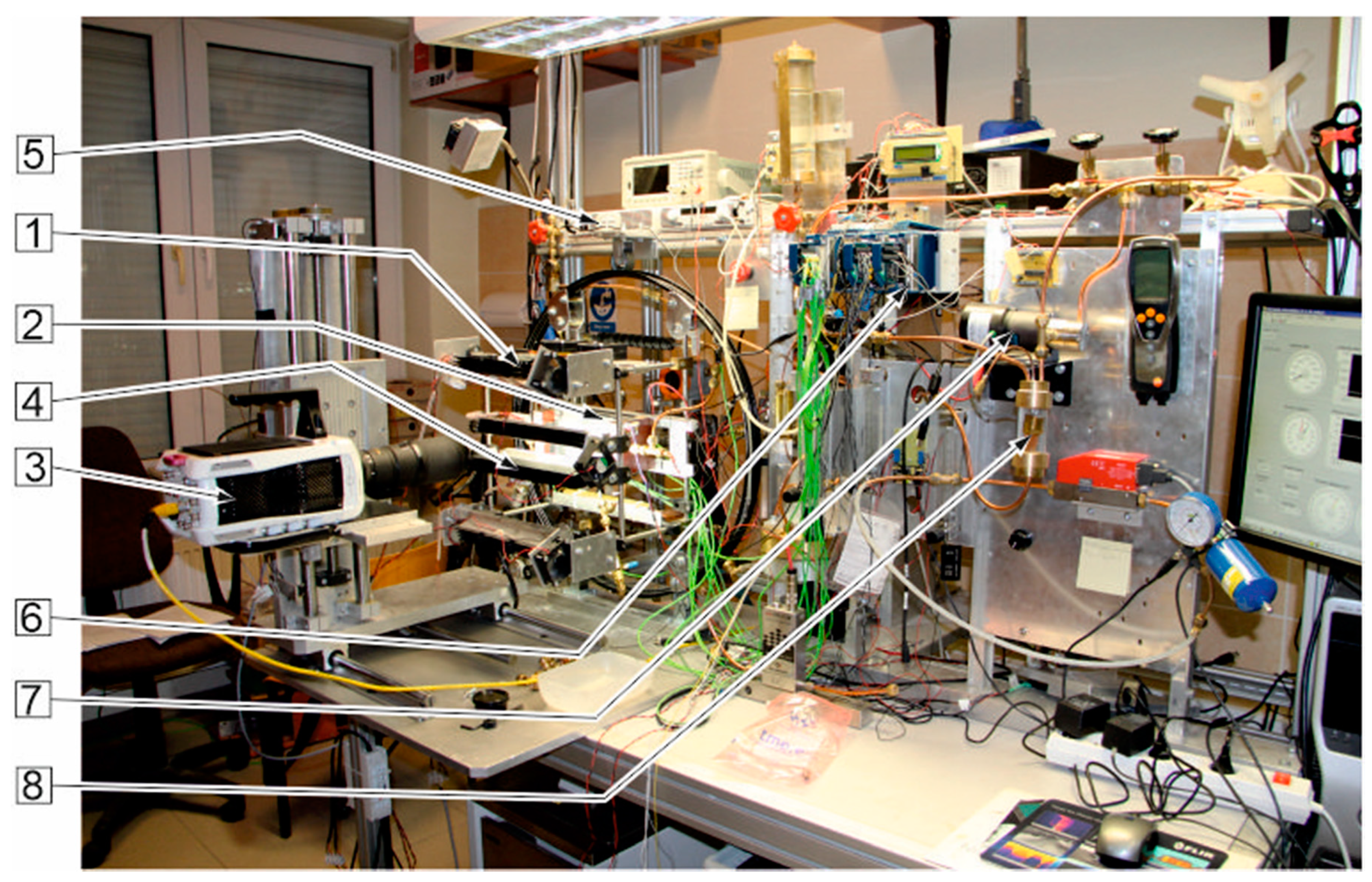
The photos in Figure 4 and Figure 5 present a general view of the experimental stand and measurement module with the mini-channel, respectively.

5. Experimental Procedure

The measurements were taken for the following ranges of the experimental parameters: total heat flux generated by four external flat heaters 129 ≤ q_t ≤ 340 kW/m² (calculated maximum error 15.4 kW/m²⁾, inlet pressure 6600 Pa ≤ p ≤ 17000 Pa, (experimental uncertainty 1250 Pa) inlet fluid subcooling 3.6 ≤ ΔT ≤ 70.7 K (experimental uncertainty 0.2 K) and mass flux 1.1 ≤ G = ≤ 8.6 kg/(m²s) (experimental uncertainty 0.26 kg/(m²s)), Reynolds number 48 ≤ Re ≤ 229.

The boiling liquid was bi-distilled, degassed water. The preset parameters were as follows:

-

Mass flux;

-

Liquid pressure and temperature at the mini-channel inlet–boiling liquid subcooling against saturation temperature;

-

Heat flux transferred to the boiling liquid.

The following parameters were measured and recorded:

-

The outlet pressure and the outlet temperature of the boiling liquid;

-

The inlet–outlet liquid pressure drop;

-

Temperature in selected points of the copper heating block;

-

Images of two-phase flow structures along the flow with high-speed film camera.

-

The obtained experimental data allowed obtaining:

-

Temperature distribution on the contact surface between the copper heater and the boiling liquid with application of the Trefftz method [20];

-

Local void fractions in the selected cross-sections of the mini-channel.

The planned starting parameters concerning the boiling liquid and the heater were set at the beginning of the experimental run. The stationary state was reached when variations of all recorded parameters, specifically the inlet liquid temperature, were negligible. The next step was setting the proper location of the film camera. The area observed by the camera was relatively small and it caused the necessity of moving the camera along the mini-channel length with fixed distances for each movement. The preset locations of the camera were in the following distances from the inlet: 0, 20, 40, 60, 80, 100, 120, 140, and 160 mm. It enabled recording two-phase flow images along the entire length of the channel L equal to 180 mm.

The computer control system precisely positioned the camera, moving it to the required location and returning to the starting point as well. Next, the recording track and number of samples for the recording were selected. During the run, the control system generated the name of the video file, containing the date, the hour, and the initial settings of the chosen parameters. Such systematic description of each video file facilitated its close assignment to the data file. The video frames were recorded in avi files at a speed of 7000 frames per second.

As a results of the experimental procedure, two files were created: one, containing the experimental data: timestamp (date, hour, minute, second, and tenth and hundredth parts of the second), both temperatures and pressures at the channel inlet and outlet, the pressure drop, volumetric flow rate and voltage drop and current supplied to the heaters; the other one, containing the video with recorded two-phase boiling flow structures in avi format, timestamped label and selected experimental data.

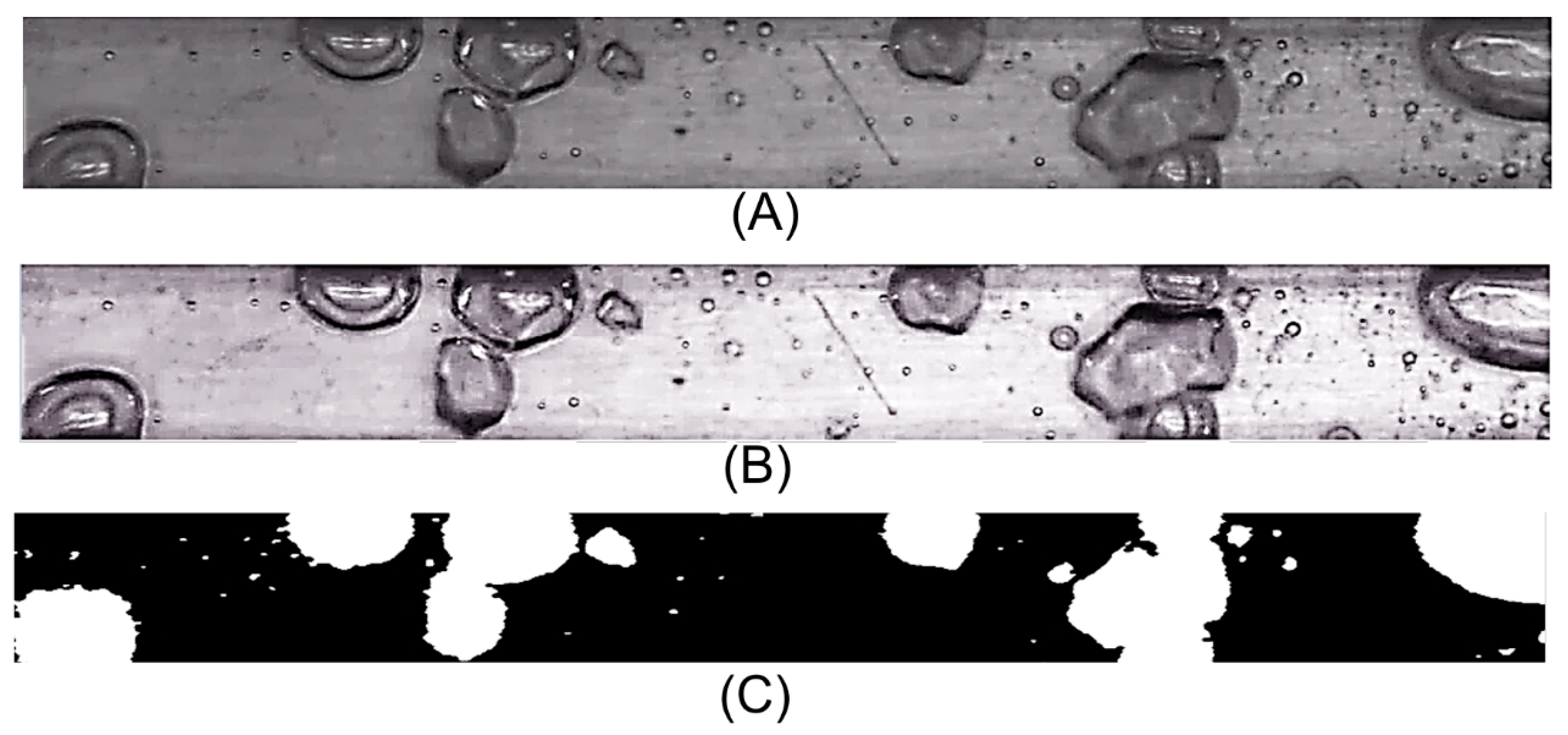
6. Flow Boiling Image Processing

Two different methods implemented in MathWorks Matlab [18] were used for vapor bubble detection and processing [21]. Observations of the boiling two-phase flow structures were the basis for selecting three characteristic bubble shapes for further investigation, as shown in Figure 6, Figure 7, Figure 8 and Figure 9. For detecting bubble shapes of type I and type II, Figure 7 and Figure 8, the Computer Vision program applied the foreground detection method, based on Gauss pixel distribution. The functions from the Image Processing Toolbox were used to detect the bubbles of shape type III, Figure 9. The functions were also used in all the mentioned cases to improve the quality of the processed image. The detector of the foreground compared the frames in their color or semi-tones of grayness with the pattern of background to determine whether the individual pixels of the frame belong to the foreground or to the background. Next, on the basis of Gauss distribution for individual pixels, the foreground binary mask was calculated.

Before calculating the void fraction, the quality of all frames was improved using operations such as frame sharpening, multiplication, and correction of contrast. Next, the refined frames were used to create the binary mask needed to perform the operations of morphological binarization, morphological opening and closing the investigated image, median filtration, and morphological filling up the empty spaces in the detected objects.

All the listed operations had to be accomplished to begin the geometric analysis with the functions implemented in Matlab. Figure 6 gives a short graphic illustration of the image refining and morphological image processing.

The geometric analysis of the refined video frames, such as those in Figure 6C, supplied the dimensions of the detected objects, namely vapor bubbles of various shapes.

It is worth noting that all linear dimensions were measured in meters or millimeters but the Matlab script read these values in pixels in each direction of the observed frame, and resolution of the image was 1280 × 156 pixels.

Each frame was indexed before the geometric analysis. Surfaces of the small bubbles, Figure 7A, and the lengths of the elongated bubbles, Figure 8A and Figure 9A, were measured.

After completing the morphological operations and binary mask generation, each refined video frame was filtered to remove the elements not belonging to the detected objects.

Next, the three-dimensional equations approximating the spatial geometry of vapor bubbles were used to convert flat images of vapor bubbles into three dimensional ones. The bubble shapes were approximated by spheres and elliptic cylinders ended with one or two ellipsoidal caps, depending on mutual relations between the dimensions of bubbles and the mini-channel, Section 6. Approximation of vapor bubble shape by a sphere or a cylinder closed with a hemisphere has previously been applied in flow boiling theoretical investigations [22,23,24,25,26,27,28]. The described procedure was used to compute void fraction in the observed fragment of the mini-channel volume. Finally, the results for each analyzed video frame were recorded in the text file.

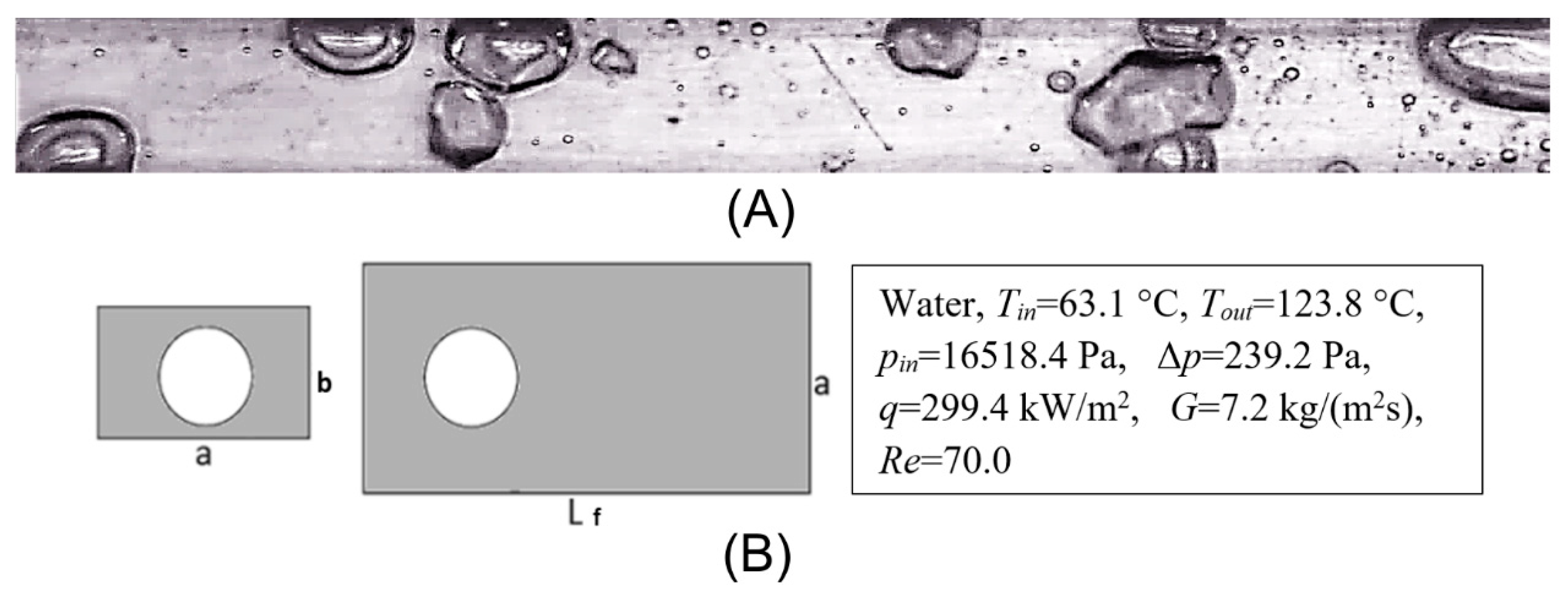
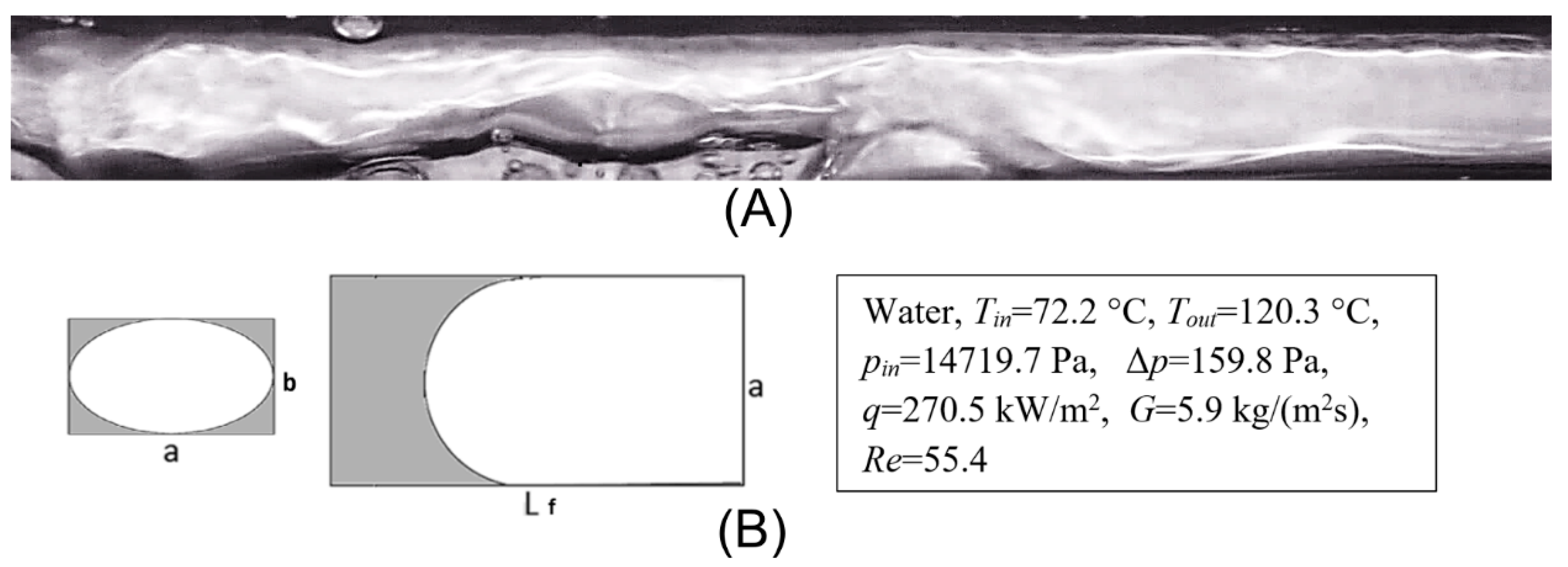
7. Computing Void Fraction

Three characteristic cases of the void fraction geometrical determination in the observed fragment of the mini-channel having the length L_f = 40 mm, width a = 4 mm, and depth b = 1.5 mm were selected and described, Figure 7, Figure 8 and Figure 9 [21]:

• Spherical vapor bubbles, R_sb,i ≤ b/2;
• Large, fully visible, elongated bubbles, with two ellipsoidal caps, semi-axes of ellipse P_1lb,i = a/2 and P_2lb,i = b/2;
• Large, partially visible, elongated bubbles, with one ellipsoidal cap, semi-axes of ellipse P_1lb,i = a/2 and P_2lb,i = b/2.

7.1. Case I

Void fraction for case I was

$${\phi }_{sb}=\frac{volume of all detected vapor bubbles}{volume of the investigated fragment of the minichannel}=\frac{4}{3Lab\sqrt{\pi }} {\displaystyle \sum }_i{A}_{sb,i}^{\frac{3}{2}}$$

(1)

where: $A_{sb,i}=\pi R_{sb,i}^2$ was the cross-sectional area of a single spherical bubble.

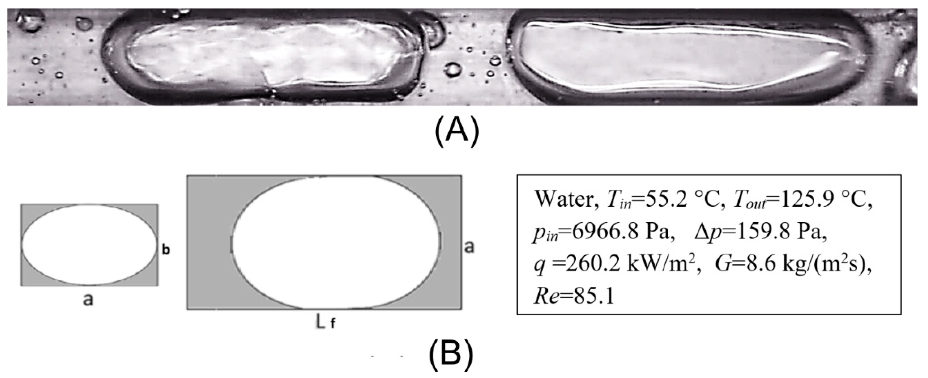
7.2. Case II

Void fraction for case II was

$${\phi }_{lb}={\displaystyle \sum }_i{\phi }_{lb,i}$$

(2)

where:

$${\phi }_{lb,i}=\frac{\left(L_{lb,i}-a\right)\frac{\pi ab}{4}+\frac{\pi a^{2}b}{6}}{Lab}$$

(3)

as the void fraction for a single elongated bubble, L_lb,i was the bubble length, composed of the length of an ellipsoidal cylinder and two ellipsoidal caps.

7.3. Case III

Void fraction for case III was

$${\phi }_{lb}={\displaystyle \sum }_i{\phi }_{lb,i}$$

(4)

where:

$${\phi }_{lb,i}=\frac{\left(L_{lb,i}-\frac{a}{2}\right)\frac{\pi ab}{4}+\frac{\pi a^{2}b}{12}}{Lab}$$

(5)

was the void fraction for a single elongated bubble; L_lb,i was the bubble length, composed of the length of an ellipsoidal cylinder and one ellipsoidal cap.

The Matlab script performed the entire procedure of recording and processing the frames and void fraction computation.

Table 1. Global scheme of the Matlab script functioning.

Selection of the Adequate Variant of the Script for the Observed Two-Phase Flow Structure, Namely for:	Spherical Vapor Bubbles Large, Elongated Bubbles, Totally Visible Large, Elongated Bubbles, Partly Non-Visible
Reading in video frames and adjustment of the internal settings of the script:	generation of the background and the object detector implementation of new settings for image processing
Enhancement of the quality of the processed video frames performance:	sharpening the video frames equalizing the brightness intensity excavation of the image details
Setting up the binary mask and exercising the following morphological operations:	image opening and image closing filling up the empty spaces in the detected objects filtration and cleaning the images from the artefacts
Analysis of the geometrical dimensions of the detected objects and application of the proper geometrical formula for:	determination of the video frame dimensions and length and area of the detected vapor bubbles indexing the detected objects matching the detected objects and right geometric formula
Void fraction calculation:	for all recorded film frames
Collecting void fraction calculation results and:	projection of the void fraction calculation results for each frame and inserting the results into a text file.

presents the summary of all sequential operations which had to be performed for each experimental run. The resulting void fraction was computed for the observed fragment of the mini-channel and averaged for the time period of the video recording, which usually took 8 s.

8. Errors of the Photographic Method

8.1. “Pixel” Void Fraction Error

One pixel was assumed to be a reasonable magnitude of linear error in measuring the radius or length of the detected bubble having the characteristic dimensions erroneously moved one pixel. The “pixel” void fraction error was based on this ground.

Table 2. Local void fraction error resulting from one pixel error in measuring the characteristic dimension of the detected bubble.

Pixel Void Fraction Error
Two-Phase Flow Structure	After Manual Segmentation	After Manual Segmentation and One Pixel Error in Measuring the Characteristic Bubble Dimension	“Pixel” Void Fraction Error ${\mathit{\epsilon }}_1=\frac{{\mathit{\phi }}_{\mathit{I}\mathit{I}}-{\mathit{\phi }}_{\mathit{I}}}{{\mathit{\phi }}_{\mathit{I}}}$
Spherical bubble	φI = 0.1372	φII = 0.1396	1.75%
Elongated, totally visible bubble	φI = 0.6855	φII = 0.6946	1.33%
Elongated, partially visible bubble	φI = 0.7969	φII = 0.8065	1.21%

compiles the representative cases of boiling two-phase flow structures and compares them forward in the flow direction. The accompanying values of the void fraction were compared in both cases as well.

The error resulting from inaccuracy of the bubble shape detection is related to manual segmentation, because it is the most precise method that eliminates detection errors made by computer scripts. The mean value of “pixel” void fraction error in Table 2 is $\overline{{\epsilon }_1}=1.43\%$.

8.2. Impact of Shadow Detection and Segmentation Procedure on Void Fraction Determination. Efficiency of the Applied Script

The shadows of the searched objects of the foreground interfere with the surroundings generating difficulties in separation, classification, and measuring the objects. Therefore, the raw video material has to be processed and reconstructed [21].

Table 3. Void fraction values after segmentation with shadow.

Two-Phase Flow Structure	Bubble with Shadow after Manual Segmentation	Bubble Detected by Matlab Script	Error of Script Segmentation with Shadow ${\mathit{\epsilon }}_2=\frac{{\mathit{\phi }}_{\mathit{I}\mathit{I}\mathit{I}}-{\mathit{\phi }}_{\mathit{I}\mathit{V}}}{{\mathit{\phi }}_{\mathit{I}\mathit{I}\mathit{I}}}$
Spherical bubble	${\phi }_{III}$ = 0.1787	${\phi }_{IV}$ = 0.1657	7.28%
Elongated, totally visible bubble	${\phi }_{III}$ = 0.7192	${\phi }_{IV}$ = 0.6964	3.17%
Elongated, partially visible bubble	${\phi }_{III}$ = 0.8080	${\phi }_{IV}$ = 0.7985	1.18%

compiles the results of the manual and Matlab script segmentation and shadow elimination. This procedure allowed the evaluation of the efficiency of the applied script.

For the two-phase flow structures considered in Table 3, the mean error of a script segmentation is $\overline{{\epsilon }_2}=3.88\%$. Therefore, the efficiency of the Matlab script in vapor bubbles detection and segmentation can be evaluated as follows:

$$\eta =100\%-\overline{\left({\epsilon }_1\right)}-\overline{\left({\epsilon }_2\right)}=94.69\%$$

(6)

The “pixel” void fraction error is well determined in contrast to the error of the script segmentation, which is difficult to precisely evaluate. The sum of both errors, namely, the mean “pixel” error and the mean error of the script segmentation is proposed as the total error of the experimental void fraction determination with the application of the discussed photographic method:

$$\epsilon =\overline{\left({\epsilon }_1\right)}+\overline{\left({\epsilon }_2\right)}=5.31\%$$

(7)

8.3. Comparison of 2D and 3D Approaches

The conversion of 2D data from the video frames into 3D is necessary to correctly evaluate the void fraction. The error of this evaluation increases when the amount of vapor in the mini-channel decreases. The examples given in

Table 4. Void fraction computed for 2D and 3D approaches.

Water
Tin, Tout, T2, T3, T4,°C	57.5; 102.7; 125.1; 124.6; 122.2	48; 89.8; 120.4; 120.3; 118.3
pin, pout, kPa	14,317.3; 14,046.6	6966.8; 6797.4
q, kW/m2; G, kg/(m2s)	333.9; 8.6	260.2; 8.6
Re; φ2D; φ3D	70.8; 31.22%; 13.37%	65.8; 50.29%; 42.5%
φ2D—φ3D/φ2D	57.2%	15.5%
Water
Tin, Tout, T2, T3, T4,°C	63.7; 103.9; 125.9; 125.4; 123.8	55.2; 103.2; 125; 124.6; 122.2
pin, pout, kPa	9751.5; 9438.8	9953.3; 9632.3
q, kW/m2; G, kg/(m2s)	333.9; 5.9	333.9; 8.6
Re; φ2D; φ3D	50; 63.99%; 58.56%	70.8; 87.95%; 80.79%
φ2D—φ3D/φ2D	8.5%	8.2%

for selected images of the boiling two-phase flow in the mini-channel before and after binarization illustrate this conclusion.

9. Selected Experimental Results. Development of the Boiling Flow Structures

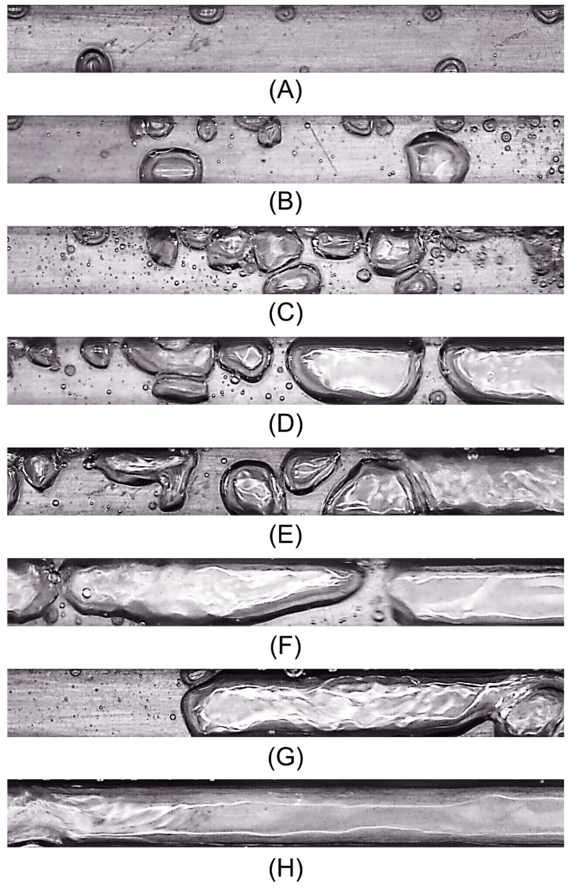
The photos below, in Figure 10, show examples of the observed two-phase flow structures that were recorded during the experimental tests.

Table 5. Thermal-flow parameters for sample structures recorded during the experiment with water, Figure 10.

Figure No.	A	B	C	D
Tin, Tout, °C	57.7; 103.1	57.5; 102.7	55.2; 97.8	63.1; 104.4
T2, T3, T4,°C	125.1; 124.7; 122.2	125.1; 124.6; 122.2	120.3; 120.2; 118.5	123.8; 123.5; 121.3
pin, pout, Pa	9751.5; 9438.8	10,234.5; 9992.5;	6966.8; 6806.9	16,518.4; 16,279.2
q, kW/m2	333.9	333.9	260.2	299.4
G, kg/(m2s)	8.6	8.6	8.6	7.2
Re	71.5	70.8	67.9	59.8
Figure No.	E	F	G	H
Tin, Tout, °C	58.2; 103.3	54,3; 102,7	68.9; 103.9	72.2; 103.9
T2, T3, T4,°C	122.8; 122.3; 120.4	125.0; 124.5; 122.1	125.9; 125.4; 123.8	125.9; 125.4; 123.8
pin, pout, Pa	12,627.7; 12,408.9	10,204.9; 9947.9	14,082.8; 13,805.2	14,719.7; 14,449.2
q, k/Wm2	299.4	333.9	333.9	333.9
G, kg/(m2s)	5.9	8.6	5.9	5.9
Re	48	70.8	50.5	50.5

compiles the basic thermal and flow parameters corresponding to the photos.

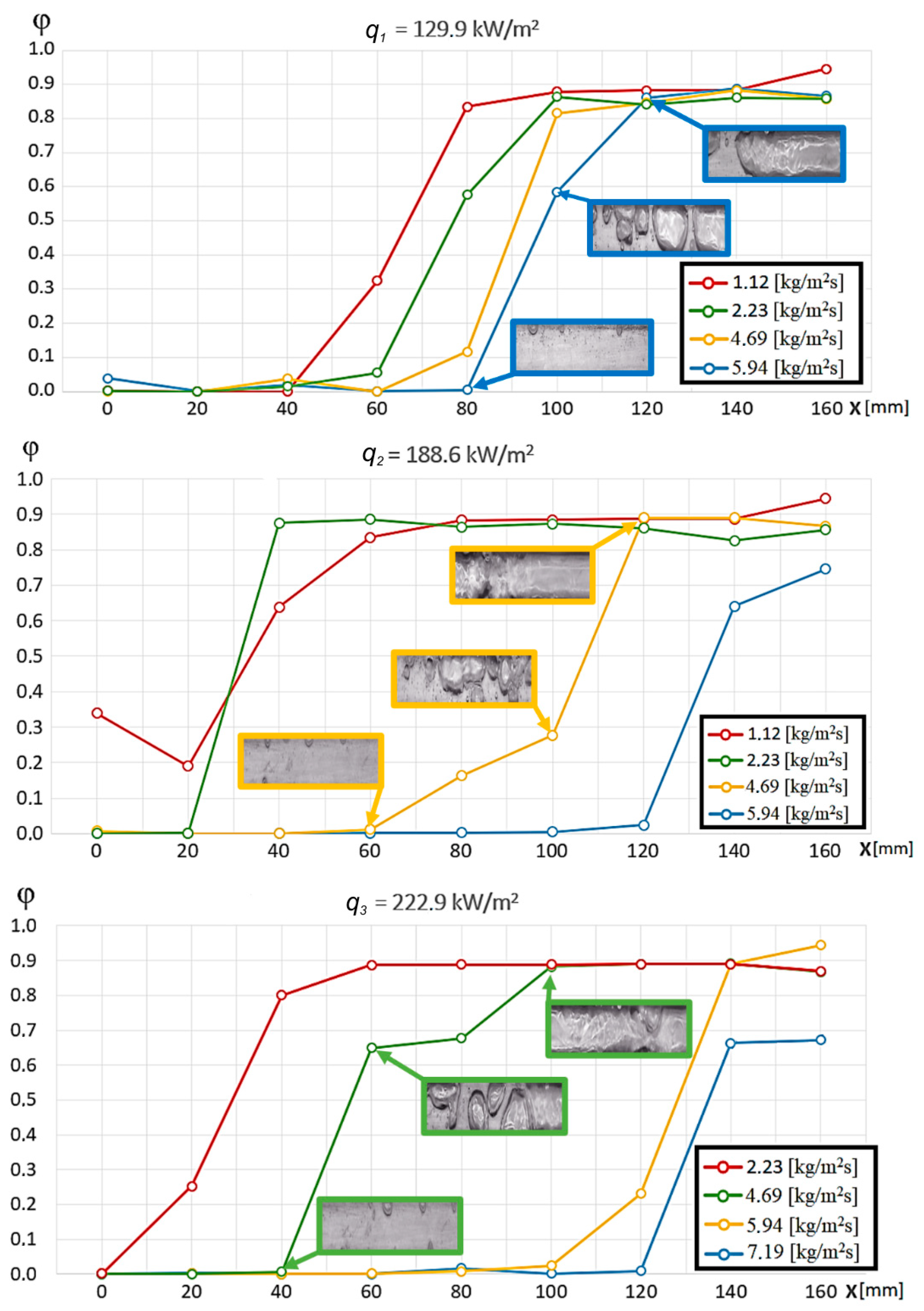
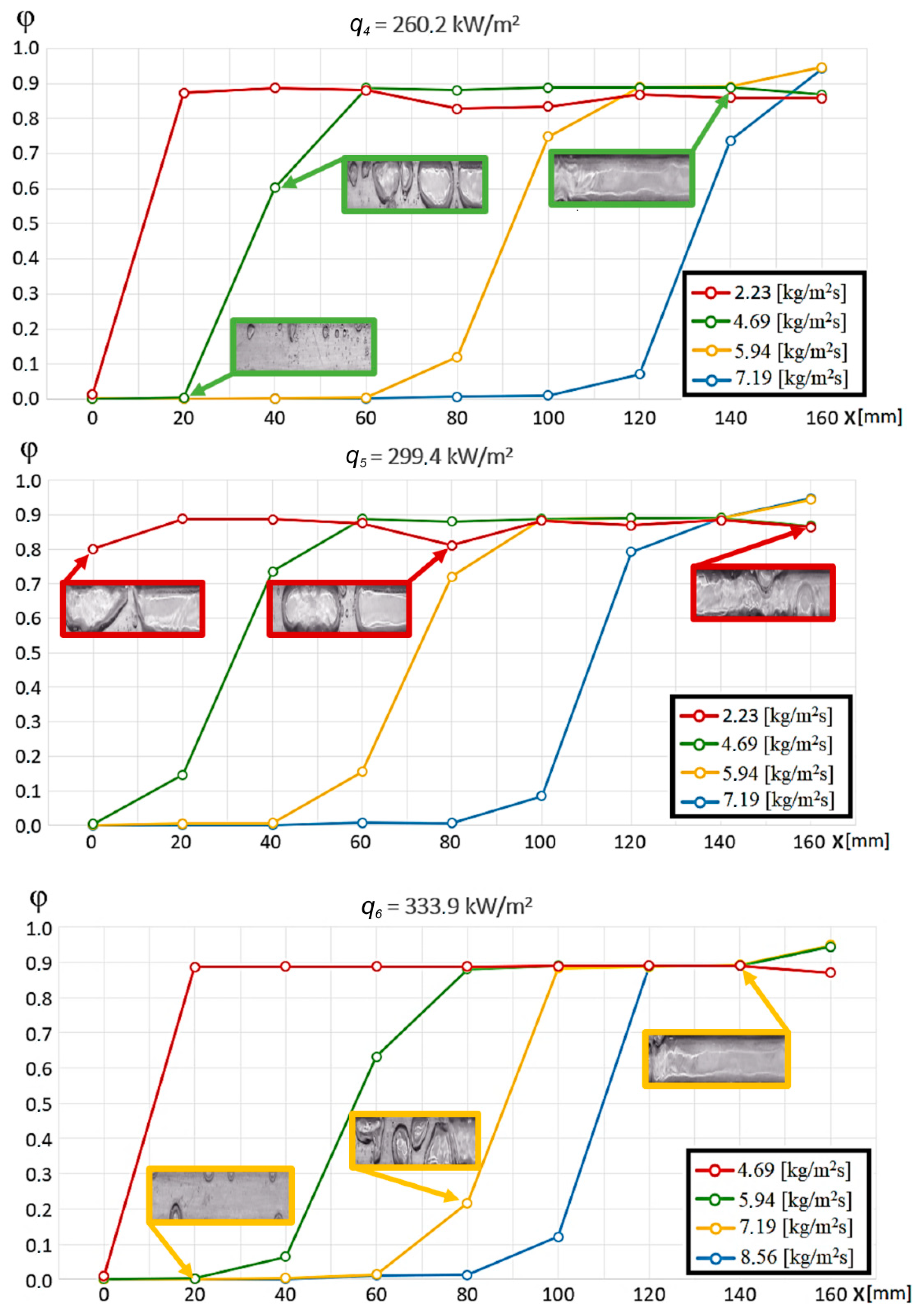
Examples of local void fraction variation along the channel length are given in Figure 11 and Figure 12. The controlled and set parameters in experimental runs were heat and mass fluxes. Inlet pressure and inlet temperature varied slightly, which is shown in

Table 6. Examples of inlet pressure and temperature variation for mass flux G = 4.69 × 10⁻⁹ kg/(m²s).

Heat Flux kW/m2	1299	1886	2229	2602	2994	3339
Tin avg, °C	72	78	75	71	74	60
Tin min, °C	67	71	70	65	68	56
Tin max, °C	79	83	81	76	77	64
pin avg, Pa	13,063	16,647	5099	5115	5283	17,415
pin min, Pa	12,301	14,949	4434	4233	4266	16,885
pin max, Pa	14,358	18,304	5391	5816	6335	18,484

.

The results obtained for the selected values of the mass and heat fluxes with camera moving along the channel length created sets of polylines shown in Figure 11 and Figure 12, each marked with different color. In the presented cases, where the mass flux was small and the heat flux was high, very intensive boiling was observed. The initiation of the boiling process was rapid and the entire mini-channel was quickly filled with vapor. In all cases observed, void fraction values rose sharply from φ = 0 at the inlet up to φ = 0.94.

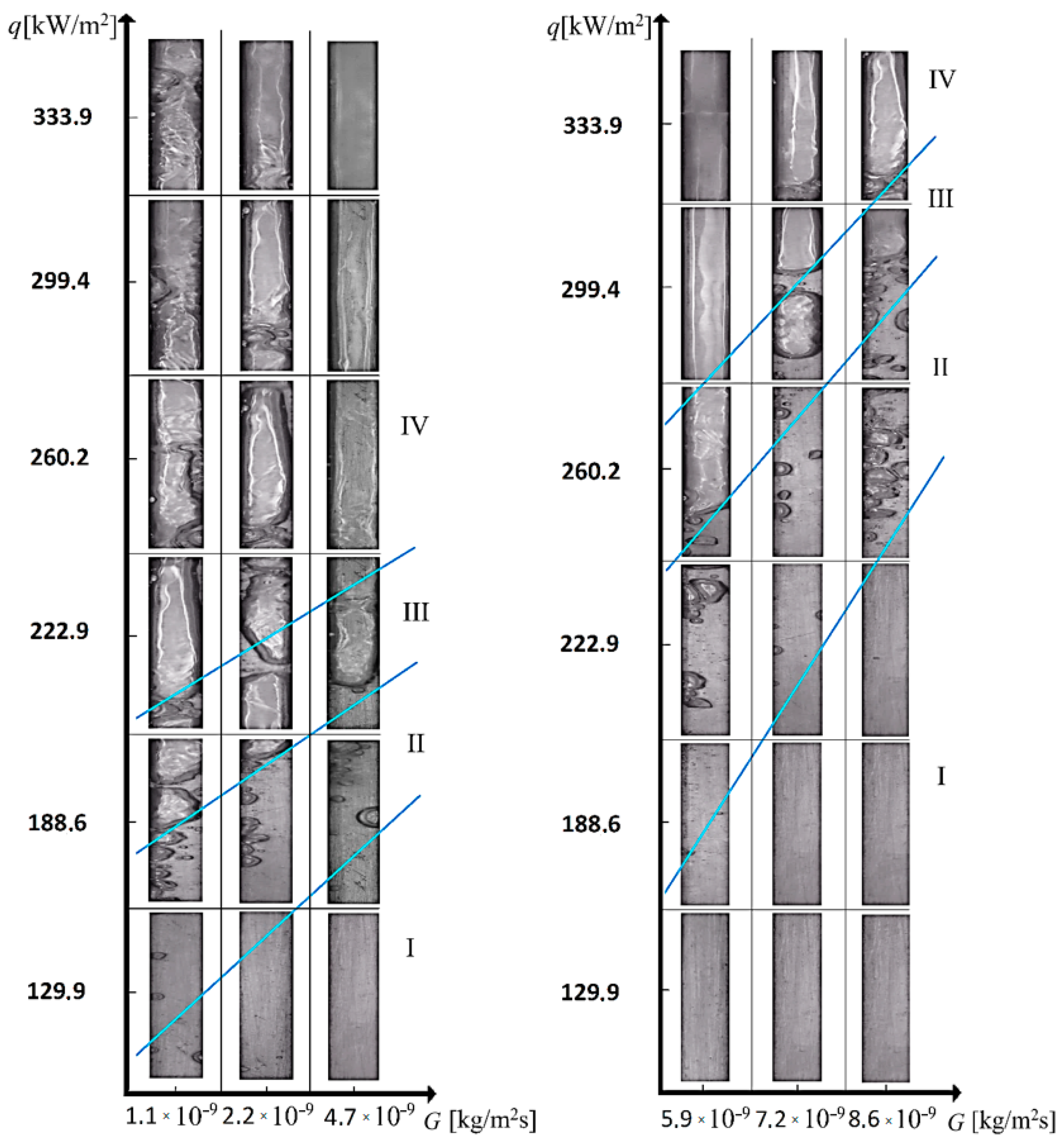
The same set of thermal-flow parameters, Figure 11 and Figure 12, was used to prepare the two-phase flow boiling maps in measured coordinates: heat flux versus mass flux, two-phase flow structure = function (q, G). The result of this approach to two-phase flow structure mapping is shown in Figure 13. The maps present the dominant and representative two-phase flow structures that occurred during the entire experiment for the given mass and heat fluxes.

10. Conclusions

Many experimental works focus mainly on using image processing methods for the analysis of two-phase flow structures as a complementary element to the study of other parameters of the boiling two-phase flow.

The experimental method proposed in this article presents a new approach to the photographic analysis of a void fraction for boiling in mini-channels with simultaneous measuring its local values and observation and recording varying two-phase flow structures. The developed method is also characterized by a small maximum error, which guarantees the high accuracy of the obtained experimental results.

The main factor limiting the use of image processing methods is the huge quantity of images collected in each experimental run which causes large time constraints. For example, in our experiments we often handled several thousand images in a single run.

The original method of approximate conversion of two-dimensional photo images into three-dimensional images of various bubble shapes was developed and implemented into the local void fraction evaluation procedure. The conversion was based on the results of the analysis of characteristic shapes of vapor bubbles encountered in the mini-channels.

Two advanced digital image processing methods were used to reduce the recorded data, namely, the background subtraction technique and the statistical analysis of individual pixel technique. Both methods were implemented in two Matlab software packages, Computer Vision and Image Processing, to obtain the final results from the photographic experiment.

In the applied photographic procedure, the total bubble segmentation error that determines the local void fraction measurement error is composed of the linear inaccuracy of the bubble dimensioning (the “pixel” error) and the script segmentation error, resulting from shadows interfering with the bubble selection and measurement. The sum values of both errors slightly exceed 5%, which seems to be a reasonable value, and, more importantly, the script efficiency reached almost 95% for dynamic flow boiling situations.

The collected experimental data were used to construct graphs showing changes of the void fraction along the length of the channel and maps of two-phase flow boiling structures. The analysis of local void fraction variations demonstrates that the development of boiling process in a mini-channel has a dynamic character. The local void fraction for most cases varied from low values (0–0.1) to very high (0.8–0.9) over the distance from 30 to 50 mm from the channel inlet. The knowledge of the local void fraction is a piece of valuable information and thus it was used by the authors to determine other flow boiling parameters [20,29].

The analysis of two-phase flow boiling maps shows that the obtained results are consistent with the expectations. Particular vapor structures form continuous areas in which the increase of vapor phase can be observed along with the increase of the heat flux. The increase of the mass flux causes the opposite tendency.

The adopted goal of combining the recording of boiling two-phase flow images with simultaneous local void fraction measurements, both based on the same photographic data set, was successfully achieved. The data reduction procedure based on Matlab with the implemented background subtraction technique and the individual pixel statistical analysis proved its efficiency in dealing with dynamically varying vapor bubble shapes.

The obtained images of the boiling two-phase flow with corresponding local values of the void fraction should ease and enhance the process of boiling flow modeling, which is still based on experimental correlations.