1. Introduction
Rechargeable Li-ion batteries are becoming ubiquitous in wide-ranging applications, such as electric vehicles, consumer electronics, power equipment and aerospace systems [
1,
2]. A battery management system (BMS) is required to ensure the safe, efficient and reliable operation of battery packs. It is quite well known that Li-ion batteries suffer from safety issues when operated outside their allowable voltage ranges. It is the task of the BMS to keep the battery within the operable range to ensure safety. A battery pack that is not properly managed is neither efficient nor reliable. For example, a pack that is not balanced is limited in its performance due to weak cells. Such cells can make the pack useless over time. Consequently, the BMS constantly monitors the battery by measuring the voltage and current of the battery to perform specific control operations [
3]. Using the measured data, the BMS accurately estimates crucial diagnostic parameters of a battery pack, such as battery equivalent circuit model parameters (ECM) [
4,
5], battery capacity [
6,
7,
8], state of charge (SOC) [
9], state of health (SOH) [
10,
11], time to shut down and the remaining useful life (RUL) [
12].
Estimation of the electrical equivalent circuit model parameters of the battery is a wide area of research. The estimated ECM parameters are used to model the voltage drop within the battery, eventually to estimate the SOC by the voltage-based approach [
13]. The estimated ECM parameters, along with the estimated SOC, can be used to compute the remaining mileage of an electric vehicle. ECM parameters determine the limits of charging current for safe and fast charging of batteries. In battery thermal management, with the identified ECM parameters, heat generated within the battery can be computed to predict the surface temperature of batteries [
14] so that it can be maintained within safe temperature limits.
Existing approaches to the estimation of ECM parameters can be broadly divided into time domain and frequency domain approaches. Time domain approaches are methods which use instantaneous voltage and current measurements to estimate ECM parameters. In the frequency domain, battery ECM parameters are estimated through electrochemical impedance spectroscopy (EIS) [
15]. EIS approach to battery ECM parameter estimation requires the application of excitation signals spanning a wide-ranging frequency spectrum, starting from a low-frequency range (fraction of a Hz) to a very high-frequency range (in the MHz range). In [
16], a nine-parameter model (2RC) was used in ECM parameter estimation in the frequency domain, resulting in moderate accuracy for only certain parameter estimates. The entire frequency scanning may take close to an hour. Frequency domain approaches have been extensively employed in battery SOH studies [
17,
18]. The EIS-based approaches have been studied generally in laboratory settings to estimate ECM parameters [
19,
20] and these approaches cannot yet be used in real-life systems. Implementation of EIS in real-life battery applications requires additional hardware in order to generate and sense high-frequency excitation signals and their responses. Time domain approaches, on the other hand, can be implemented without requiring special excitation signals, which will be the focus of this paper.
The literature on time domain approaches generally considers the co-estimation of ECM parameters and the SOC [
21,
22] of battery. For example, in [
23], parameter estimation for four different equivalent models of the battery, that represent typical battery operation modes, were discussed. For the four models, joint linear parameter estimation and SOC tracking framework were proposed. This approach is faced with dependencies on the knowledge of k-parameters of the open-circuit voltage (OCV)—the state of charge representation, i.e., OCV-SOC parameters of the battery. Additionally, the estimation of SOC is usually subject to errors in SOC initialization, integration and uncertainty in the knowledge of battery capacity. Such SOC errors consequently translate to errors in the estimation of ECM parameters using the co-estimation approach. The persistence of these errors can also be seen in methods that model battery parameters as a function of the SOC [
24]. When the internal battery impedances are modelled as a function of the SOC, an extended Kalman filter (EKF) is generally implemented to jointly estimate SOC and the other battery parameters. Further, different identification methods such as the EKF, particle swarm optimization (PSO) and recursive least square (RLS) are discussed in [
25] to estimate the battery’s internal ECM parameters along with SOC. In [
26], higher accuracy is achieved by retaining initial values for less important parameters and updating the parameters relevant to SOC and SOH estimation. It can be said that time-domain approaches to estimating ECM model parameters of a battery, without requiring other battery state information, remain sparse. In [
27], an approach to independently estimate ECM parameters without requiring the SOC is proposed, where the observation model was developed based on the differentials of voltage and current measurements. However, the possibility of estimation of OCV as one of the parameters is not considered. Further, theoretical performance bounds in the accuracy of estimation were not derived.
Cramer–Rao lower bound (CRLB) defines the theoretical minimum estimation error variance, i.e., the theoretical performance bound that an estimator can achieve. In this paper, it is shown that the CRLB of estimation has a dependency on the choice of current profile for accurate estimation of internal open-circuit voltage and resistance of the battery. Using this, better approaches can be developed for ECM parameter estimation by optimizing the voltage-current profiles. Different works on ECM parameter estimation have considered different current profiles for the estimation of battery parameters [
28]. However, in these works, it is neither shown that the profiles are optimal for the estimation of parameters nor is an approach to relating the estimation accuracy to the preferred current profile derived.
The contributions of the present paper are as follows:
ECM parameter estimation without the knowledge of SOC: In this paper, ECM parameter estimation is formulated as a linear least squares estimation problem. Using the proposed approach, the internal open circuit voltage and the ECM parameters can be estimated without depending on the OCV-SOC model parameters and the SOC estimation algorithms, which are potential sources of errors that can eventually affect the identification of the battery’s internal impedance. The developed approach is a simplistic model in terms of the voltage and current measurements from a battery.
Theoretical performance analysis: The theoretical analysis is completed for the proposed approach using the theoretical bounds of estimation Cramer–Rao lower bound (CRLB). The CRLB defines the relationship of the estimation accuracy with regard to the measurement noise characteristics, the number of observations and the current profile.
Current profile optimization or improved estimation accuracy: It is shown in this paper that the CRLB takes a simplified closed form for the simple R-int model of the battery. While it is known that the estimation accuracy improves with lower measurement noise variance and more observations, avenues are opened to explore current profiles that minimize the CRLB of estimation.
Optimization approach to select the current profile: For the first time, an optimization approach is developed that describes the selection of current profiles to improve the accuracy of estimation. It is shown that a pulse current of equal charging and discharging magnitude minimizes the CRLB in the estimation of both the internal open circuit voltage and the internal resistance of the R-int model of the battery.
The approach presented in this paper is demonstrated using a battery simulator developed in MATLAB and validated on experimental data collected from a commercial battery.
The remainder of the paper is structured as follows: In
Section 2, the mathematical derivation of the new measurement model that is based only on the measured voltage and current through the battery is presented. In
Section 3, the derivation of the measurement model is extended to different model orders.
Section 4 describes the proposed parameter estimation method and
Section 5 contains the theoretical performance analysis of the proposed method.
Section 6 summarizes the results of the testing approaches for simulated and real data.
Section 7 concludes the paper.
2. Signal Model of a Battery
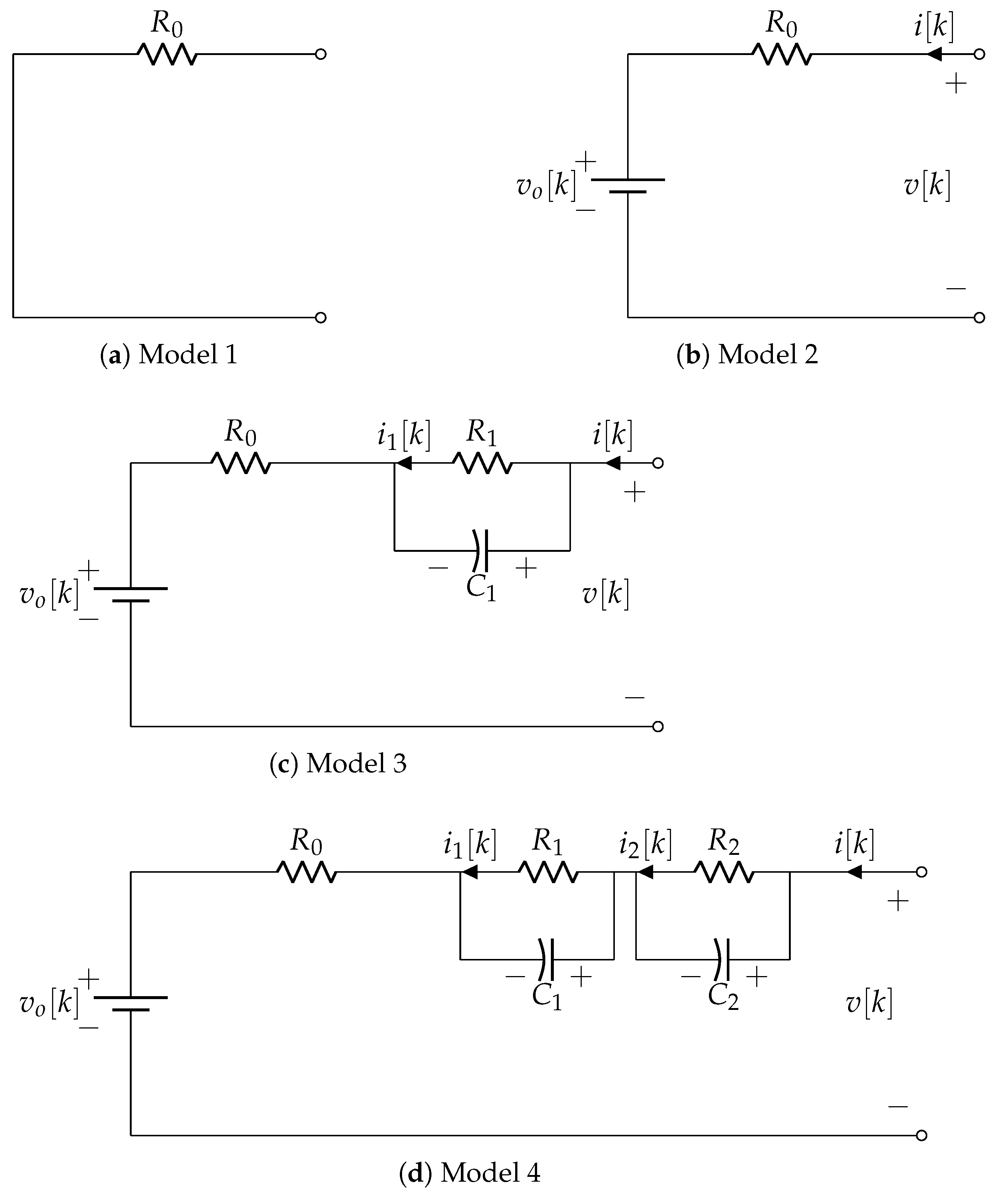
Figure 1 shows four different approximations of an ECM to be considered in this paper. Model 1 represents a short-circuited battery; a detailed analysis of Model 1 parameter estimation can be found in [
5]. Model 2 represents the R-int model and is the subject of this paper. Models 3 and 4 represent higher-order and more accurate representations of a battery. Unlike Models 1 and 2, the optimal linear approach to parameter estimation is not feasible in Models 2 and 3. The derivations presented in this section are based on the most general model shown in
Figure 1d.
Section 3 shows how these derivations can be applied to the other three models.
The measured current through the battery is written as
where
is the true current through the battery and
is the current measurement noise which is assumed to be zero mean and has a standard deviation (s.d.)
The measured voltage across the battery is
where
is the true voltage across the battery and
is the voltage measurement noise which is assumed to be zero mean with s.d.
.
For the ECM model in
Figure 1d, the true voltage across the battery,
, is written as the sum of the voltage drop across the internal components,
,
,
and the EMF,
. Hence, (
2), can be rewritten as,
where the currents through the resistors
and
can be written in the following form
where
and
is the sampling interval. By substituting the measured current
for
, the currents in (
4) and (
5) can be rewritten as follows
Now, using (
1), (
3) can be rewritten in the
z domain as follows
Next, let us rewrite (
8) in the
z domain
which yields
and similarly for (
9),
By substituting (
12) and (
13) into (
10), one gets
Rearranging (
14) and converting it back to the time domain, we get
where
Consider
to be constant over a small window of time
k; then,
. Therefore, (
15) can rewritten as
Now, let us rewrite (
16) in the following form
where the observation model
and the model parameter vector
for the ECM model are given by
The subscripts 4 in (
18) and (
19) indicate that the model corresponds to Model 4, as in
Figure 1d. Equivalent circuit models 1–3 are discussed later in
Section 3. The noise in the voltage drop in (
17) is written as
which has the following autocorrelation
This autocorrelation
for different values of
l are given below:
All the noise auto-correlation values can be summarized as follows:
4. Parameter Estimation Method
The measurements are grouped into batches of equal length
. Using (
26), the vector observation model is rewritten for a particular batch of data of length
.
where
denotes the batch number,
The correlation matrix of the noise vector
is written as
where
is a banded symmetric Toeplitz matrix which is diagonal for Models 1 and 2, tridiagonal for Model 3 and pentadiagonal for Model 4. The diagonal entry of
is given by
, the first off-diagonal entry is given by
and the second off-diagonal entry is given by
in (
29) to (
31). All the other off-diagonal elements of
are zero.
Given the
batch of observations, the least square (LS) estimate of
can be written as
It can be shown that the covariance of the LS estimation error is
When the parameter
needs to be estimated using more data, the batch length
increases, resulting in significantly high computational complexity. Rather than increasing
, a recursive least square (RLS) algorithm can be employed to achieve the same performance without significantly increasing computational load. Algorithm 1 summarizes one iteration of the RLS algorithm. The input to this algorithm is the estimate
and the error covariance
from the prior batch, the new measurement
and the new measurement model
. The outputs are the new estimate
and the updated error covariance
| Algorithm 1 |
- 1:
Update residual covariance:
- 2:
Update gain:
- 3:
Update parameter:
- 4:
Update information:
|
The calculation of the model parameters from the estimates
is given below for Model 3. From (
28), the estimate has four elements:
After estimation, the parameters of the ECM Model 3,
and
are recovered as follows:
5. Performance Analysis
In this section, a theoretical performance analysis of the proposed parameter estimation algorithm is developed. For linear observation model (
32) under Gaussian noise assumption, the Cramer–Rao Lower Bound (CRLB) [
29] serves as the lower bound on the estimation error covariance. It can be shown that, for the observation model (
32), the CRLB is
i.e.,
where
denotes an estimate of
Now, let us focus on the CRLB corresponding to Model 2 in
Figure 1 for an in-depth analysis. For this model, the CRLB simplifies to
and
can be expanded as follows
where
is assumed in order to simplify the analysis.
Now,
can be simplified as
where
From the above, the CRLB of estimating
and
, the first and second diagonal elements, respectively, of (
38) can be written as
In other words, one can write
Let us first consider
in (
42). The estimation accuracy depends on the following three factors:
- (1)
Measurement noise variance The lower the measurement noise, the lower the CRLB.
- (2)
Number of observations L. Under the given assumptions, that remains a constant, more measurements will decrease estimation error.
- (3)
Current profile The current profile should be selected in a way that the error bound in (
42) is minimized.
Out of the three factors influencing the estimation error of , two are constants. The current profile should be selected in a way that the error can be made as small as possible.
Remark 1. Let us assume all the values of the current are the same, i.e., . This will make the denominator of (42) zero and lead to infinite error variance. Another way to look at it is that all equal values of will make rank deficient. We need to find the current profile such that the can be reduced. The problem can be formally stated as follows:
Problem 1. For a given number of measurements L find such that the following cost function is maximized: under the constraint that It can be shown that for given values of the current limits and , a current profile that alternates between the two extreme values will minimize .
Minimization of can be formulated as the following problem:
Problem 2. For a given number of measurements L, find such that the following cost function is minimized: under the constraint that Selecting current limits such that
and a current profile that alternates between
and
will minimize both
and
.
The performance analysis presented in this section shows that the accuracy of the estimation depends on the excitation signal. By carefully selecting the excitation signal, the accuracy of ECM parameter estimation can be improved. When there is no control over the excitation signal, e.g., when using battery usage data for ECM parameter estimation, the CRLB provides the lower bound on the ECM parameter estimation error.
6. Simulation Analysis
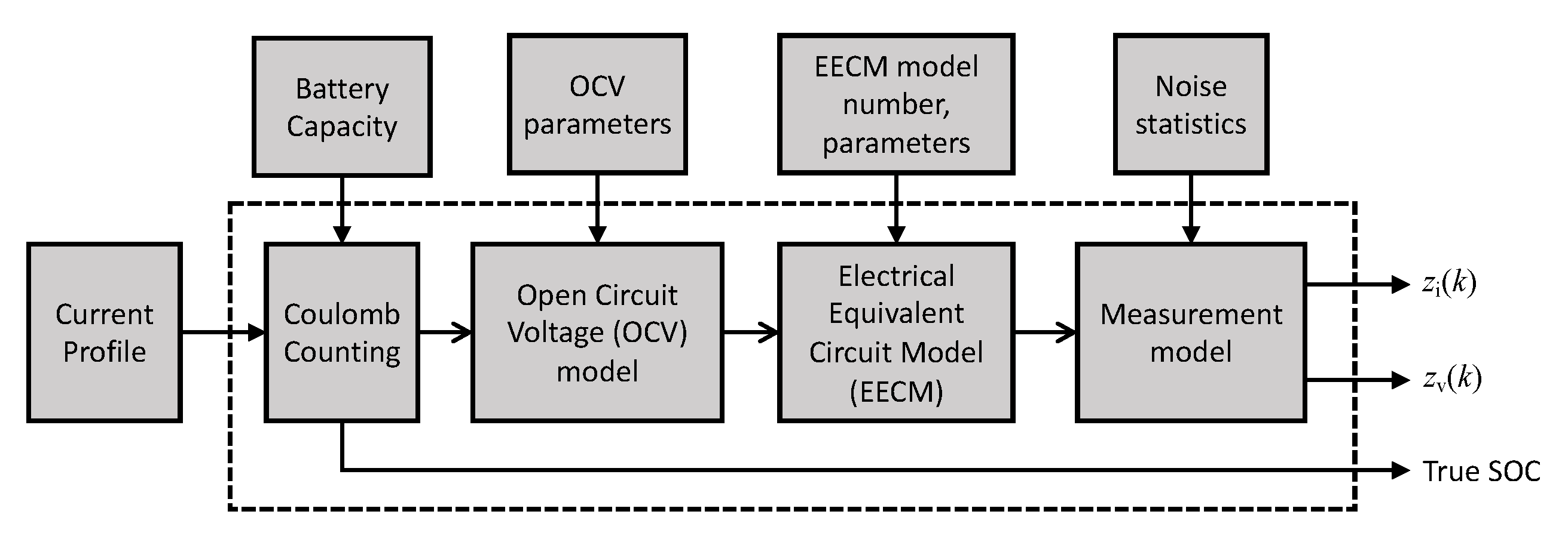
The data for the demonstration in this section were generated using a battery simulator.
Figure 2 shows the battery simulator in the form of a block diagram. The battery simulator uses the equivalent circuit model shown in
Figure 1 to simulate the voltage and current measurements that resemble real-time measurements from a battery. All simulation analyses in this paper were done by using MATLAB software version R2022a developed by MathWorks [
30]. The OCV effect of the battery, denoted by
in
Figure 1, was generated using the Combined+3 model [
31] with the following model parameters:
and
The voltage measurements across the battery were simulated using the observation model in (
3). The voltage and current measurement noises were implemented based on (
2) and (
1), respectively, where the voltage and current measurement noise standard deviations were assumed to be equal in magnitude, i.e.,
, where
was computed based on the assumed signal-to-noise ratio of the measurement system, defined as
where
is the amplitude of the current signal that is assumed to be constant throughout the entire simulation. The relaxation parameters of the ECM are set at
and
. The EECM model in the battery simulator can be changed in a way that the RC models can be selected from the set of
.
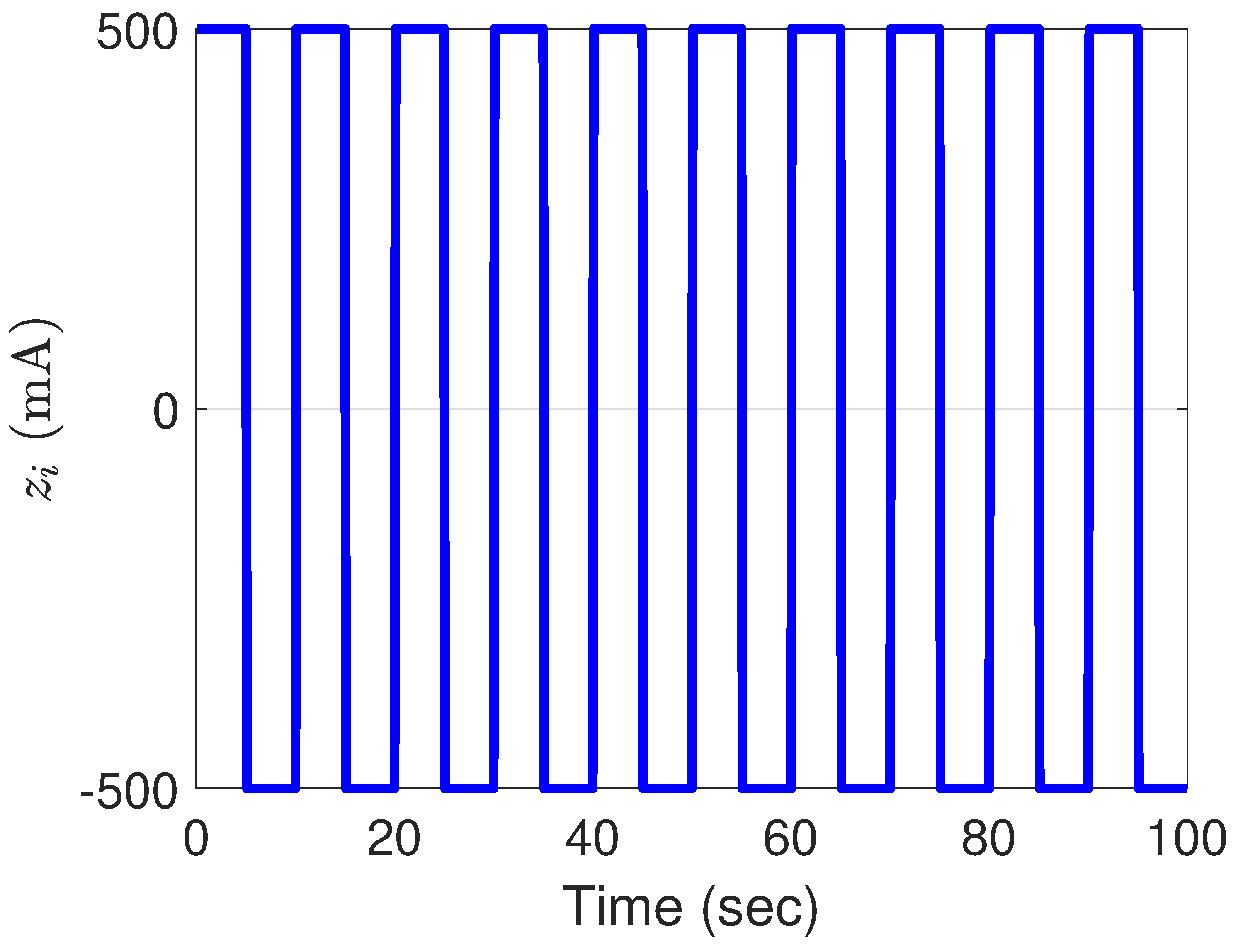
First, let us consider the current profile shown in
Figure 3. The current is sampled at
resulting in
samples. The current profile
also holds the following property
where
.
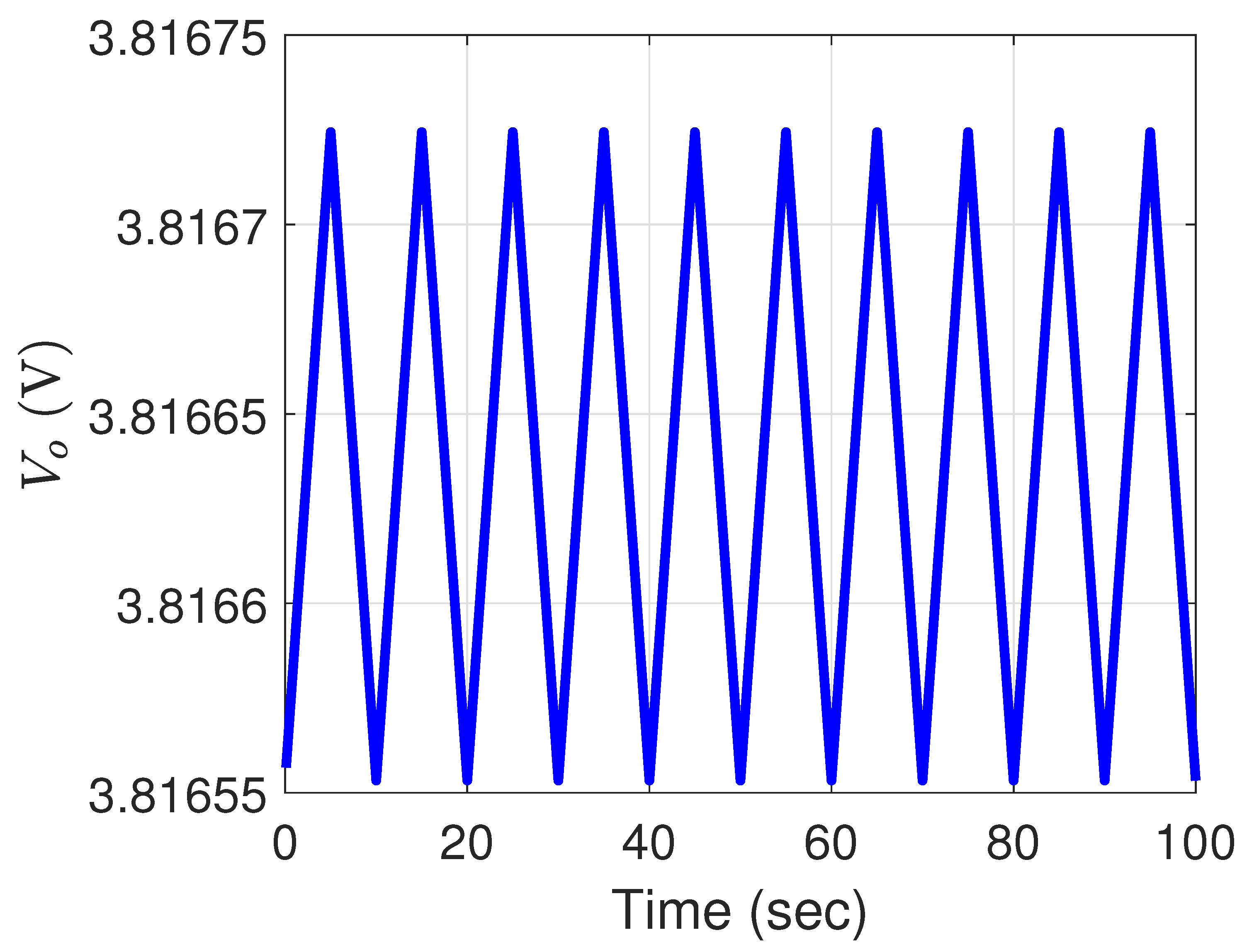
Figure 4 shows a plot of OCV
over time. It can be seen that when the current
is positive
increases and when
is negative
decreases. Since the average current shown in
Figure 3 is zero, the average OCV in
Figure 4 is constant as well.
Figure 5 shows a plot of the true voltage across the battery terminals,
over time. It must be noted that even though
changes with time, the magnitude of the voltage drop
remains a constant. Moreover, the magnitude of change in
(see
Figure 4) is relatively insignificant compared to the magnitude of
. Consequently, the magnitude of
appears unchanged in
Figure 5. Another explanation for this observation is that the change in OCV is small within a duration of 5 s.
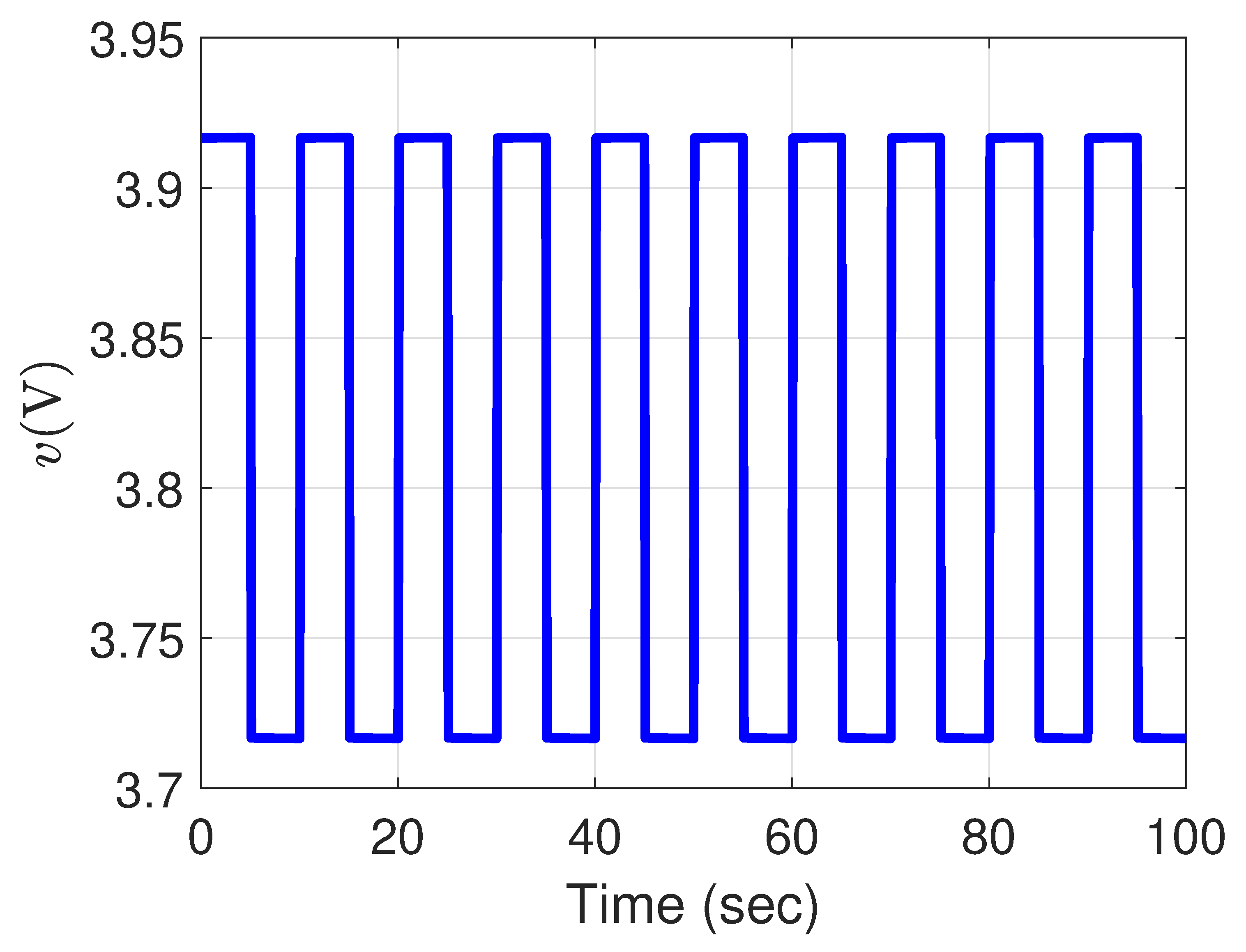
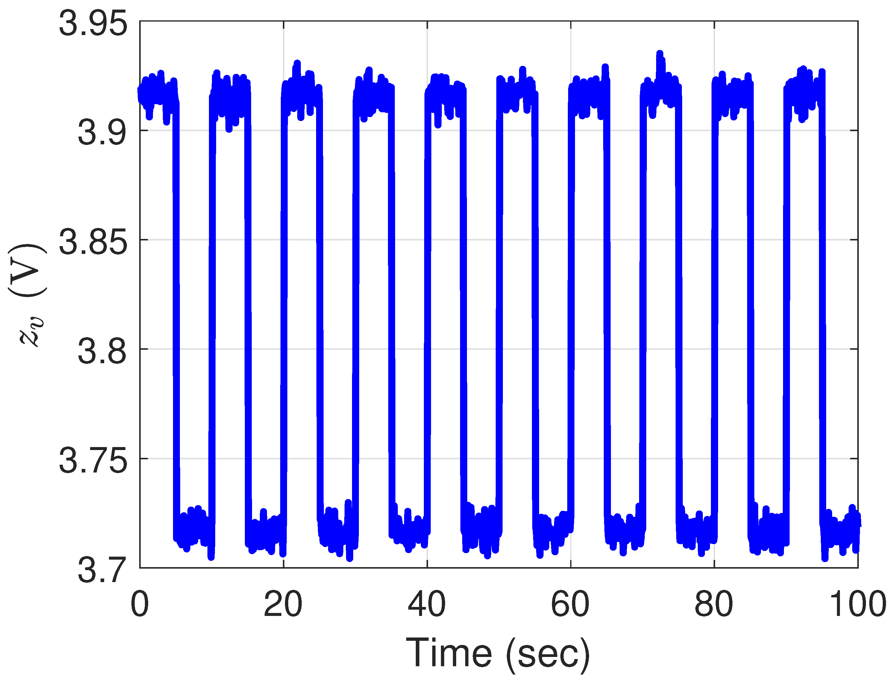
Figure 6 shows the voltage measurements from the battery simulator. Here, the battery simulator is set to Model 2 ECM (see
Figure 1), i.e., only
had a non-zero value and all other ECM parameters were set to zero. For now, it is assumed that the current profile is perfectly known, as shown in
Figure 3; i.e., it is assumed that the current measurement noise is zero.
The least-square estimation algorithm (
34) for Model 2 was used to estimate the resistance
and
. Let us denote these estimated quantities as
and
, respectively. The normalized mean square error (NMSE) of these estimates is defined as
where
M denotes the number of Monte-Carlo runs.
In order to make the CRLB comparable to the NMSE defined in (
52) and (
53), the following CRLB values in (
42) and (
43) were computed for comparison during simulation studies.
6.1. Perfect ECM Assumption
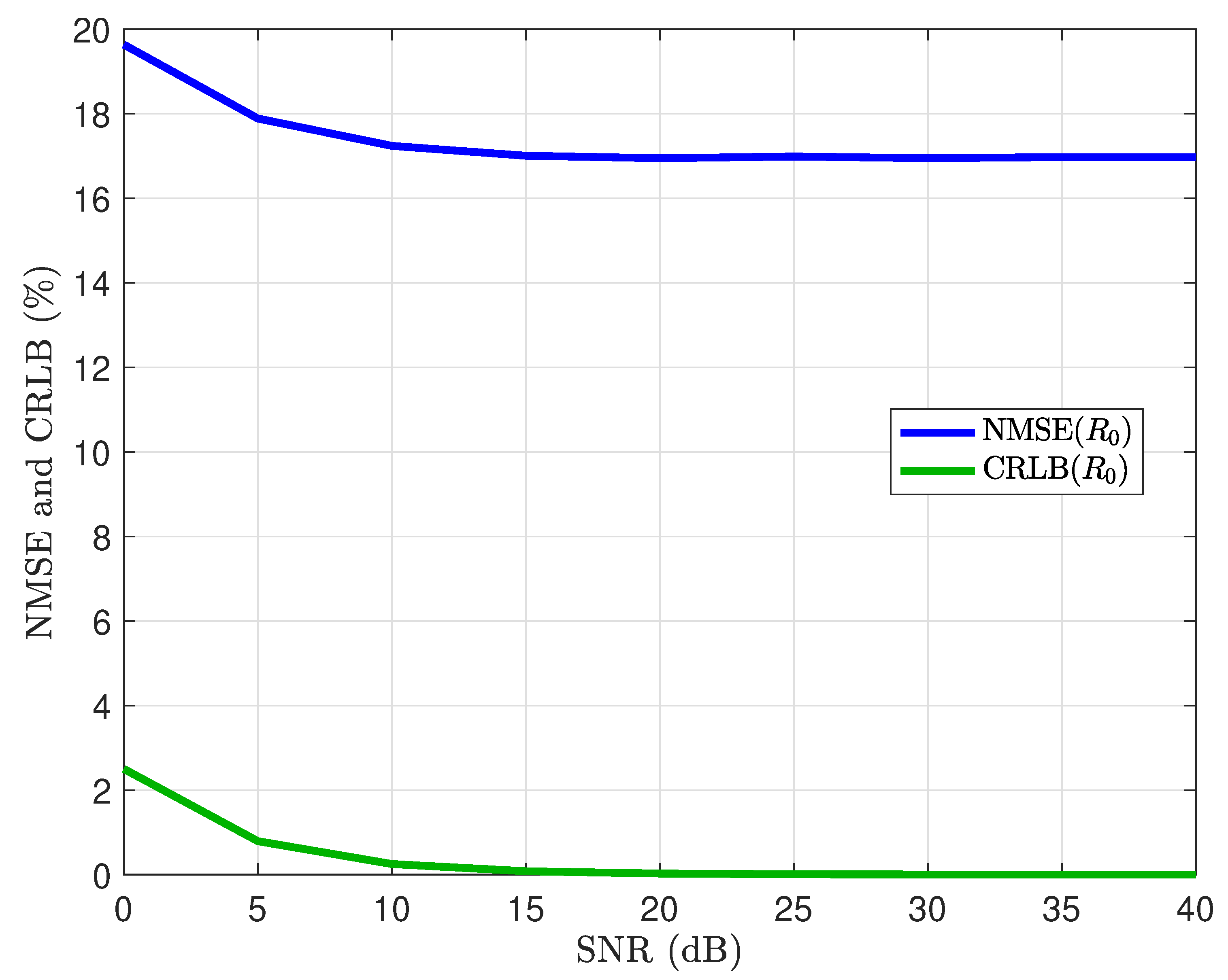
In a perfect ECM assumption, the battery management system assumes the same model as the battery simulator. We will now consider a scenario where the battery simulator and BMS assume Model 2. The NMSE for
is calculated using Equation (
52) where
for Model 2 is estimated over 1000 Monte-Carlo runs. The CRLB for
is calculated using Equation (
54), where the length of current samples (
Figure 3) is
.
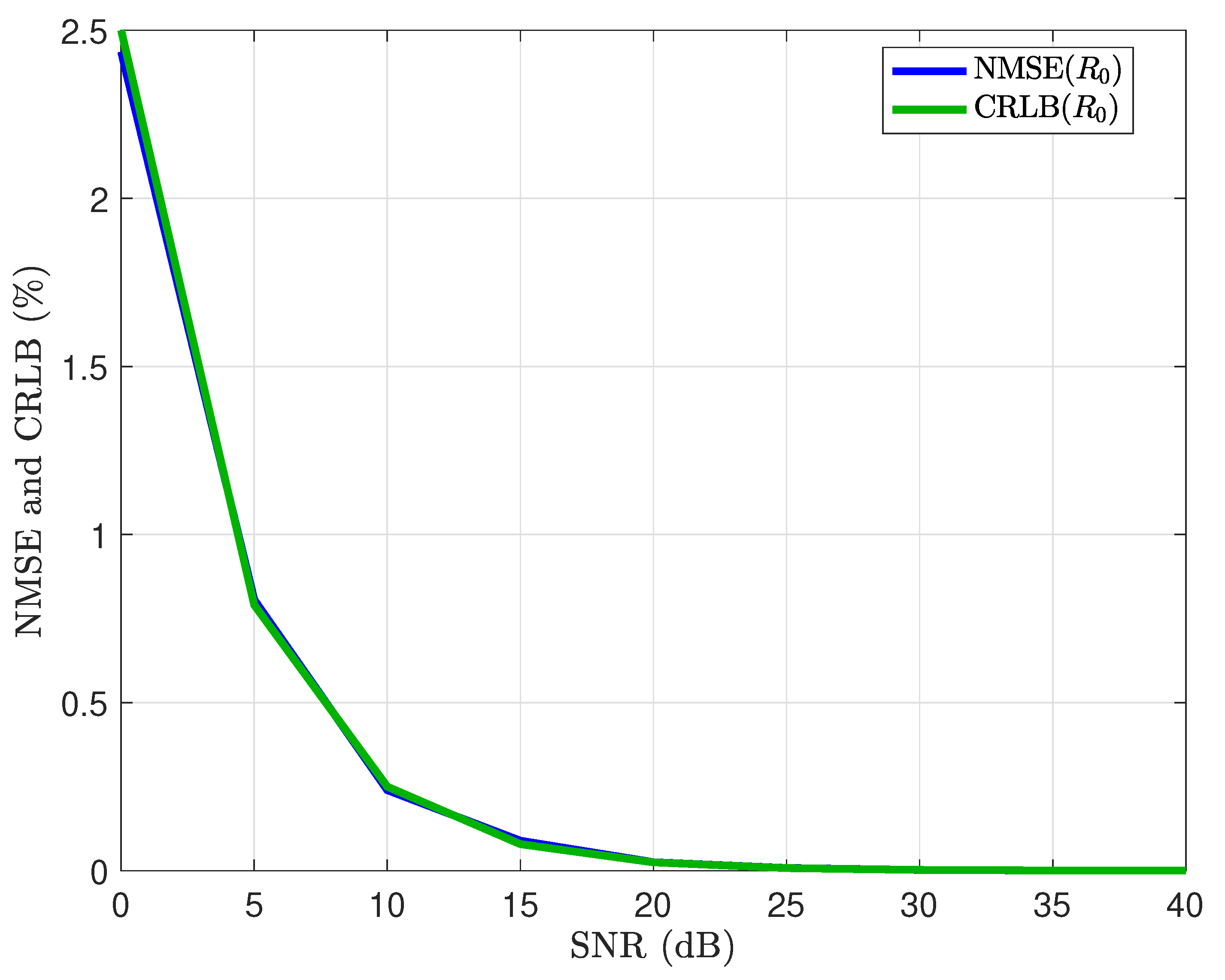
Figure 7 shows the NMSE and CRLB for
estimation under model matched assumption. It can be observed that the NMSE is close to the theoretical bound CRLB for all SNR levels indicating an efficient estimator.
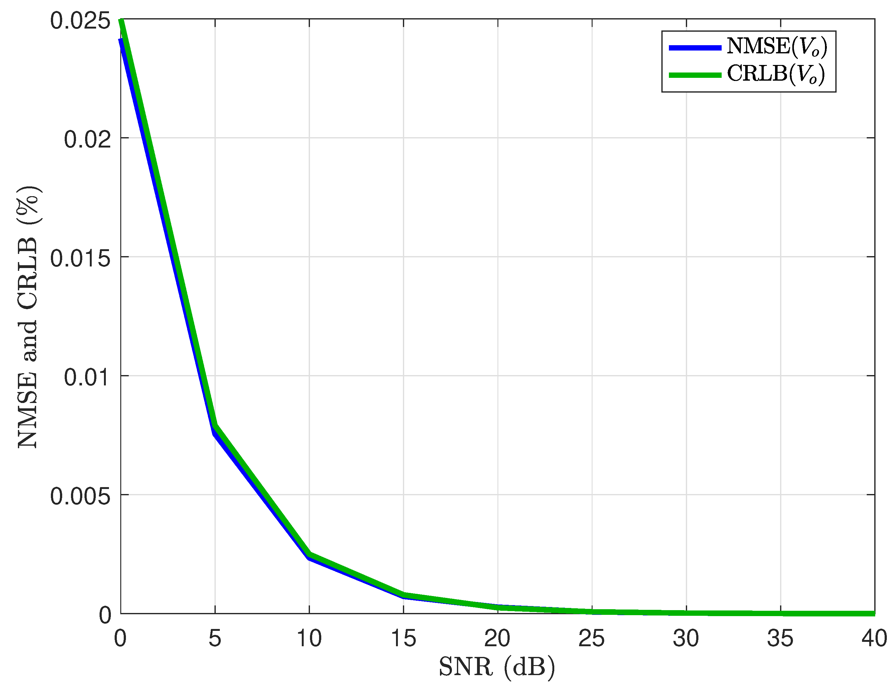
Similarly, in
Figure 8, the NMSE of
estimate is plotted with CRLB of
for SNR values between 0 and 40 dB. The NMSE of
estimate is calculated using (
53) and the CRLB of
estimate is calculated using (
55). It can be observed again that the performance of the estimator is close to the theoretical bound CRLB and that the estimator is efficient.
Now, let us compare the resistance estimates under the perfect ECM assumption for a particular SNR level.
Table 1 contains the
estimate for Model 2 under perfect ECM assumption at SNR = 20 dB. When the BMS and battery simulator assumes Model 2, the estimate of resistance
is obtained as an average from the estimate of
over 1000 Monte-Carlo runs. The table also shows another case of perfect ECM assumption where the simulator, as well as the estimator, correspond to Model 3. Due to this assumption, the model parameter vector consists of two resistance
and
values as in
Figure 1c. Thus, when the BMS and battery simulator assumes Model 3, the estimate of resistances,
and
are obtained as an average from the estimates of
and
over 1000 Monte-Carlo runs.
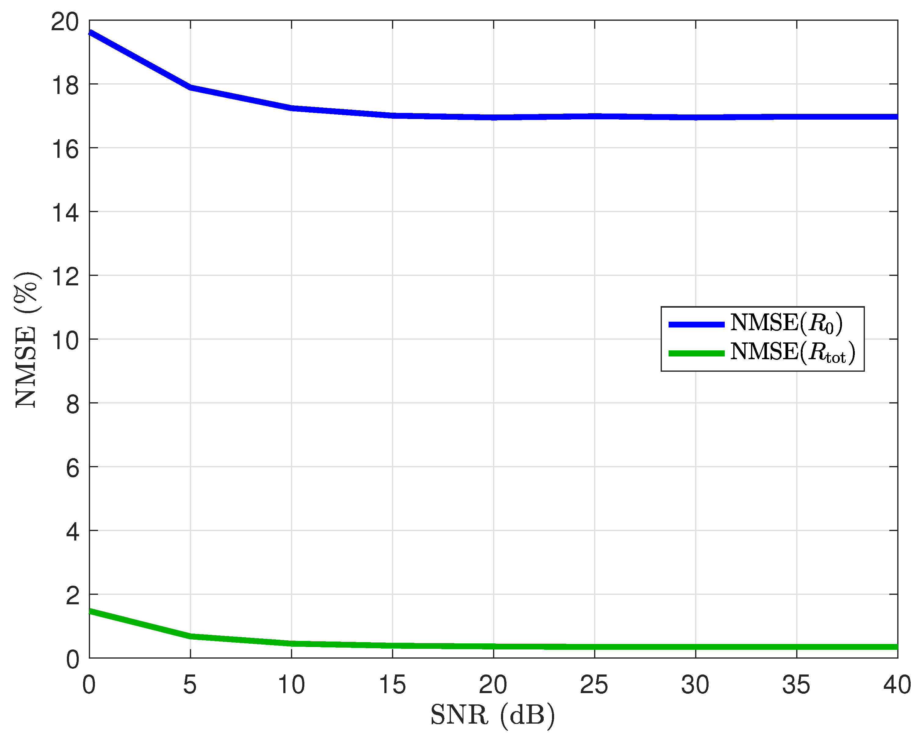
6.2. Realistic ECM Assumption
In this section, a simulation-based ECM parameter estimation analysis is presented based on a realistic ECM assumption in which the battery management system assumes an ECM model that is different from the one used by the battery simulator to simulate the measurements. In this section, we consider a scenario where the battery simulator assumes Model 3 and the BMS assumes Model 2. It must be noted that the CRLB derivations are done under perfect model assumptions.
Figure 9 shows the NMSE and CRLB computed under the model mismatch assumption. The NMSE is significantly greater than CRLB at all SNR levels. An explanation for this observation can be stated based on the model assumptions made for this simulation: ECM Model 3 contains two resistor components,
and
. When a lower order model, here Model 2, is used to estimate the parameters, the resulting estimate of the resistance is observed to be closer to the sum of the two resistor components of Model 3. To confirm this observation, let us define a new type of NMSE as follows:
Here, the estimation error is computed with respect to the total resistance, defined as
Figure 10 shows the computed NMSE based on the two different definitions given in (
52) and (
56). In this figure, it can be observed that
is less than the NMSE for
at all SNR levels. This means that the BMS under the Model 2 assumption estimates both resistances together, as a summation. Thus, it can be confirmed that the estimation of resistance of ECM Model 2 is approximately the sum of the two resistor components of Model 3.
Now, let us compare the estimates of resistances under the perfect and realistic ECM assumptions at a particular SNR level.
Table 2 contains the averages of the
and
estimates for both assumptions of ECM Model 3. The parameter estimate is obtained as an average from the estimates of 1000 Monte-Carlo runs at SNR = 20 dB. While using the realistic ECM model, the estimation algorithm assumes a different model, Model 2. Thus, from the ECM in
Figure 1b, one estimate of resistance is obtained, i.e.,
. Now we apply the observation that the resistance of an ECM Model 2 is approximately the sum of the two resistor components of Model 3. Conforming to this observation, the Model 2 estimate is shown to be the total resistance of ECM Model 3
under perfect ECM assumption.
The simulation analysis presented in this section under realistic ECM assumption is important because of the fact that when it comes to real battery applications, the assumed model is always different from the realistic case. Moreover, most battery management systems resort to reduced order models in order to save computation and hardware complexity.
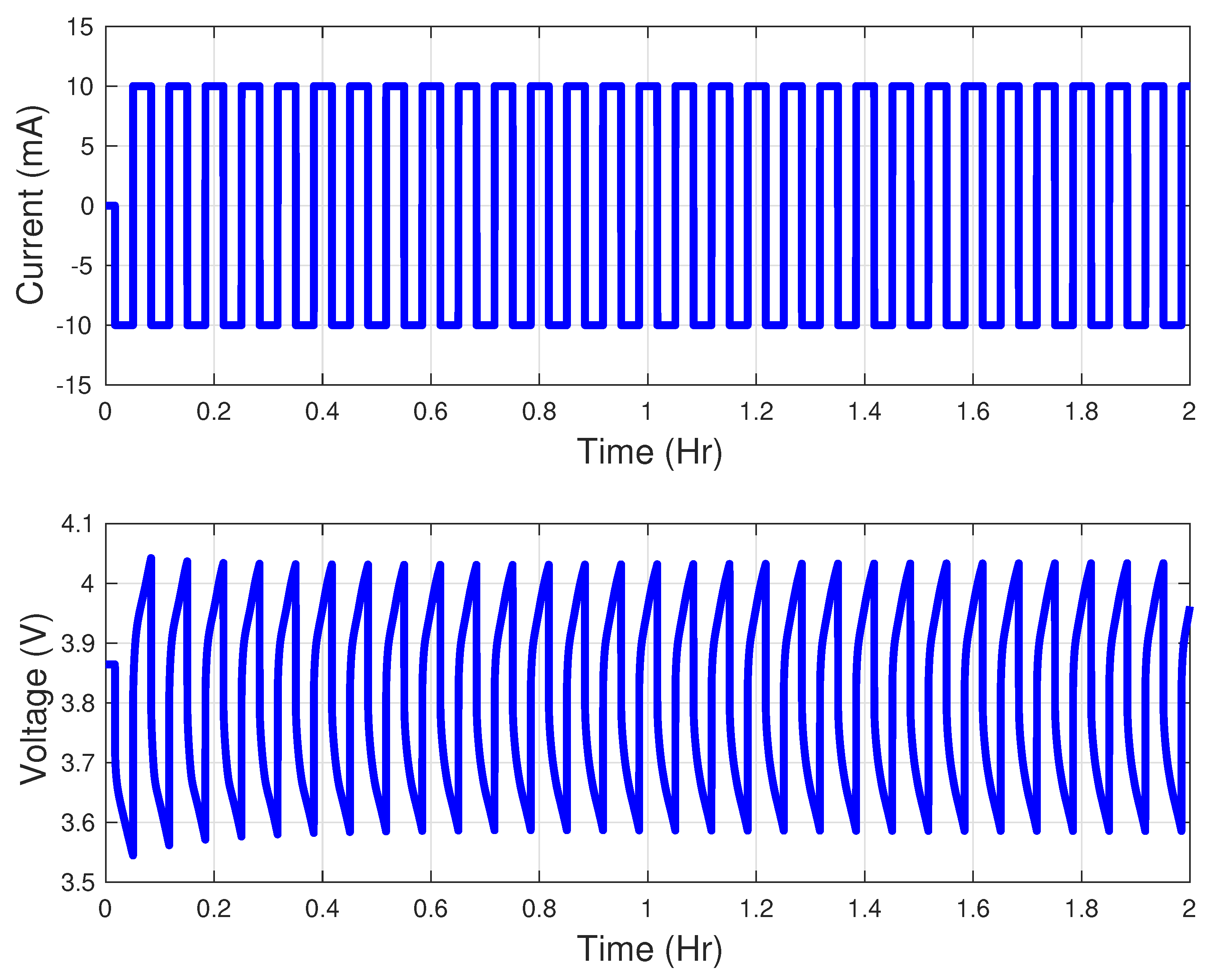
6.3. Real Data
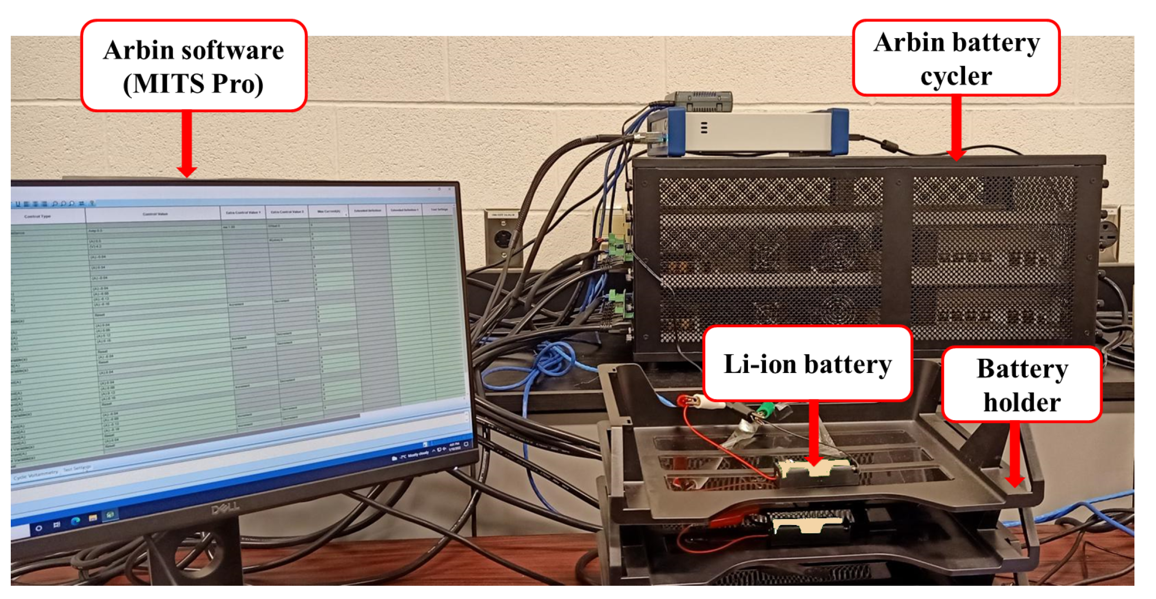
In this subsection, the performance of the proposed approach for battery parameter estimation using data collected from a Samsung-30T INR21700 battery cell is presented. A current profile, shown in
Figure 11 is applied to the battery and the voltage across the battery terminals is recorded. The data collection is performed using the Arbin BT-2000 battery cycler shown in
Figure 12 and is made available in this link:
https://data.mendeley.com/datasets/h3yfxtwkjz, accessed on 24 October 2022.
The s.d. of the voltage and current measurement error of the device is approximately
and
, respectively. The sampling time of the data is
second; this resulted in close to 7200 voltage and current measurements as shown in
Figure 11. Then, least square estimation (
34) is performed on the recorded data to estimate the model parameters.
Table 3 shows the parameters obtained when the estimation algorithm is set to ECM Models 2 and 3, respectively. The parameter estimate is obtained as an average from the estimates over 1000 Monte-Carlo runs. Here, while using Model 2 to estimate the parameters, the resistance estimate is
. When Model 3 is used, the individual resistance estimates are
and
, resulting in
, which is approximately equal to the Model 2 estimation of
Thus, the observation that while using Model 2, the resistance obtained is closer to the summation of all the resistor components of Model 3 holds true for real-battery data.


