1. Introduction
Biomass is a carbon-neutral and clean source of energy. The amount of carbon dioxide produced during combustion is absorbed by crops during photosynthesis [
1,
2]. Further, biomass is abundant and renewable and can be found everywhere from trees to animal waste. Globally, each year, over one billion tons of agricultural material (wheat, grain, corn, etc.) are wasted [
3], which can potentially provide billions of tons of producer gas. In spite of all the advantages of biomass, according to data from the U.S. Energy Information Administration (EIA) on April 2022, only about 4.7% of all energy consumption in the United States is from biomass energy production [
4].
To increase the share of biomass in energy production, the fluidization hydrodynamic behavior of these particles must truly be understood. The profile of biomass particles can change drastically from very fine grains to very long and thin particles. Biomass particles in general are irregular in shape, size, density, and pliability and have low sphericity, which could lead to problems in fluidization, such as particle agglomeration, elutriation, and segregation [
5]. To address these issues, a secondary inert material, such as sand or alumina, can be added to the bed. However, the significant differences in the properties of biomass and inert particles can lead to a non-uniform distribution of biomass particles within the fluidized bed. This can cause major issues with particle interactions and mixing. Hence, gaining enough knowledge about the successful fluidization of biomass particles alone is crucial and can be used in different industrial applications. For this purpose, numerical models have been proven to be a powerful tool. Eulerian–Eulerian models as opposed to Lagrangian models allow for modeling large industrial systems. Eulerian–Eulerian models treat both phases as an interpenetrating continuum, and the kinetic theory for granular flows (KTGF) is used to model the solids phase constitutive equations. Due to their nature, biomass particles have a tendency for agglomeration. However, KTGF only explains the motion of particles and not the particle clusters. Hence, various closure laws have been proposed to improve the performance of Eulerian-Eulerian models with KTGF to successfully predict the fluidization behavior of this group of particles. Choosing a set of granular models and properties that are adaptable to biomass particles with their irregular properties is crucial in reliable simulations. There is some research focused on the effects of particle irregularities on fluidization behavior and how to address this issue to successfully predict the hydrodynamics of the process using Eulerian–Eulerian models.
Since the effect of these irregularities presents itself on the drag force exerted by the fluid phase on the particles, some researchers focused on drag models. Nikku et al. [
6] applied a characterization method of an average drag force combined with the results of an imaging analysis performed using a commercial image analysis software. The method was applied to four different materials, and the results were compared with the data of a single particle drag. The results demonstrated that irregularly shaped particles must be approached in a different manner when it comes to their size and shape. It was found that considering all dimensions of the particles as well as applying the characterization method as a way to describe these particles was critical for determining the average gas–solid drag force. Later, Hua et al. [
7] proposed a new drag model that switches between the Ganser correlation in the dilute solid concentration condition and the Ergun correlation in the dense condition. Using the proposed drag model, Hua et al. [
7] conducted a Eulerian–Eulerian CFD model to predict the fluidization behaviors of irregular Geldart B particles, and validated their results with a lab-scale experiment. The proposed drag model effectively predicted the behavior of the particles, while it was found to be sufficiently stable to the slight changes of
and
. They also proposed a method to accurately estimate particle sphericity using
and
and suggested that this method accompanying the proposed drag model was a reasonable and convenient way to predict the fluidization behavior of irregular particles using Eulerian–Eulerian models. Estejab and Battaglia [
8] studied the effect of drag models on the fluidization behavior of biomass particles and their mixtures. They studied an assortment of drag models to improve the simulation of the hydrodynamics of fluidization behavior. They found that for Geldart A biomass particles, for both single and binary phase mixtures, the Gidaspow-blend drag model yielded the best results compared to experimental data, that is, if the static regions that do not participate in fluidization are considered.
To understand the effects of particle irregularities, some studies tested different simulation methods and some focused on the important parameters. Elfasakhany and Bai [
9] studied the motion of irregularly shaped biomass particles in turbulent flows both numerically and experimentally. In order to computationally model the flow of particles, both one- and two-way coupling were employed for two-phase flows. In one-way coupling, the fluid continuum affects solid particles via drag and turbulence, but the reverse effect was not considered. In two-way coupling, however, the interaction occurs both ways, meaning both phases affect one another. In addition, they proposed a shape function to account for the irregulates of particles studied. It was found that the use of the shape function was crucial to successfully predict the fluidization behavior of irregularly shaped particles yielding no significant differences between the one-way and two-way coupling. Hence, it was proposed that one-way coupling is sufficient to successfully predict the fluidization behavior of biomass particles. Subsequently, Girimonte et al. [
10] studied the fluidization of binary mixtures of irregularly shaped biomass mixed with inert particles. The results indicated that the theoretical models for determining the characteristic fluidization velocities of two spherical solids in a binary mixture, including initial and final fluidization velocity, can, in fact, be extended to binary mixtures of irregularly shaped particles. It should be noted that the conclusion above was made by applying sphericity to correct the particle size used in the developed equations. Through the theoretical equations, an optimal size of the inert particles to promote the biomass distribution along the bed height was also concluded. Consequently, better mixing of components in the bed was achieved. Later, Rashid et al. [
11] computationally researched the effects of the following three granular solid properties in a two-phase riser in the fast fluidization regime: granular viscosity, frictional viscosity, and solid pressure. The studied particles were categorized as Geldart A and Geldart B particles, and the sub-grid drag model was employed. The simulations of the Geldart A particles aligned well with the experimental results. However, the simulations of the Geldart B particles significantly differed from the experimental results at higher heights, whereas the change of solid granular properties had negligible effects on the results at lower heights. Rashid et al. [
11] also concluded that it is necessary to apply the turbulent model for the fast fluidization regime, where simply assuming laminar flow predicted unrealistic results.
Cáceres-Martínez et al. [
12] studied the importance of the physical properties of biomass particles on the determination of the minimum fluidization velocity,
. They used various biomasses to test the accuracy of the correlation reported in the literature to find
. In all the cases tested, sand was present as the inert, and diverse mass ratios of sand-biomass were considered. However, the highest biomass mass ratio in the mixture tested was 10%. The significant impact of particle size, particle sphericity, and the mass fraction of the biomass in the bed on the fluidization of the mixtures was reported along with the observed importance of the Geldart classification on the satisfactory performance of correlation reported in the literature to find
. He et al. [
13] reviewed the agglomeration of biomass particles in a fluidized bed. In their review, they attributed biomass agglomeration to the existence of inorganic elements in the chemical composition of biomass. The review specifically focused on the impact of various types of alkali salts on biomass agglomeration. It was found that alkali salts behave differently throughout the fluidization process and have varying effects on the agglomeration of biomass.
The properties of irregularly shaped particles deeply impact the fluidization process. In order to successfully consider these irregularities in computer modeling, some researchers have proposed new shape functions [
9], while others have sought to explain the effects by proposing new drag models or modifying commonly used ones [
6,
7]. Additionally, some researchers have suggested adjusting experimental data in computer codes to achieve accurate simulation results [
8,
14]. While some researchers have studied the effects of different functions embedded in Eulerian–Eulerian models [
11], there is still a lack of research on finding models that prevail in predicting the fluidization behavior of irregularly shaped particles. Models, depending on their structure, perform differently when applied to various shapes and sizes of particles. The novel aspect of this research is to examine these effects and identify the models that excel in predicting the fluidization behavior of irregularly shaped particles by solely using sphericity as the shape function and commonly used drag models. The outcomes of this research will help improving simulation results by identifying the most adaptable models for biomass particles. This research will specifically focus on varying granular properties, including radial distribution functions (RDF), frictional viscosity models (FVM), angles of internal friction (
), and stress-blending functions (SBF) for irregular biomass particles of Geldart B. The results of this study will present the best combination of models and properties to accurately predict the fluidization behavior of biomass particles while considering the randomness in properties. Throughout the course of this research, a Eulerian–Eulerian model with embedded KTGF called Multiphase Flow with Interphase eXchanges (MFIX) will be employed. To the best of the authors’ knowledge, no prior studies have specifically focused on embedded functions in MFIX to determine the most effective models that can accurately predict the fluidization behavior of irregularly shaped biomass particles without the need for adjusting experimental data, while utilizing a simple shape function (sphericity) and a commonly used drag model. The simulation predictions are compared with experiments [
5] when possible. The experimental data, which was obtained through a series of 2D X-Ray imaging that were subsequently constructed into a 3D image [
5], was used to validate the results of the current study. This paper makes significant contributions to the investigation of the impact of irregularly shaped particles on the fluidization process. The objective is to identify the most suitable models for predicting the fluidization behavior of irregular biomass particles.
3. Results and Discussions
In order to successfully consider the irregularities of biomass particles in computer modeling, researchers have suggested different solutions, such as developing new shape functions [
9], proposing new drag models or modifying commonly used ones [
6,
7], and adjusting experimental data to be used in computer codes [
8,
14]. However, the results of this study reveal that by selecting the right functions embedded in Eulerian–Eulerian models, these adjustments are unnecessary. The performance of models can vary greatly depending on their structure when applied to particles of different shapes and sizes. The preset research examines these effects and identifies the models that excel in predicting the fluidization behavior of irregularly-shaped particles, relying solely on sphericity as the shape function and commonly used drag models. Ultimately, the results determine the most adaptable models to biomass particles and the best combination of models and properties, which can significantly improve the simulation results. This research will specifically focus on exploring the variation of granular properties, including radial distribution functions (RDF), frictional viscosity models (FVM), angles of internal friction (
), and stress-blending functions (SBF) for irregular biomass particles.
Biomass particles have a broad profile, from very fine grains to very long and thin particles, and consequently they have a high tendency to clump together and create agglomeration during the fluidization process. The particle irregularities also affect the orientation of particles in the reactor, where non-spherical particles can reside in the bed at different angles. This can affect the average distance between particles in the bed, and as a result, can influence the size and location of voidages in the bed. Hence, void fraction and solids volume fractions in binary beds are influenced greatly by particle irregularities. Consequently, the changes in solid volume fraction affect the gas velocity, where gas particles’ path and speed are dictated by the dynamics of the bed. Gas particles pass through the granular bed of material by detecting easy paths; therefore, particles agglomeration and clumps hinder the gas flow. Further, the drag force exerted on the particles is a function of particle shape and the way that a particle resides in the bed. Hence, the solid velocity is also influenced by particle irregularities. The shape and size of particles also affect the bulk density of the bed of material, which influences the pressure drop across the bed. In this section, the effects of different models on each one of these properties are discussed.
3.1. Effects of RDFs and FVMs
3.1.1. Effects of RDFs and FVMs on Void Fraction
To study the effects of different RDFs and FVMs on the performance of irregularly shaped biomass particles, simulation predictions are investigated and compared to the results of experiments from Deza et al. [
5] when possible.
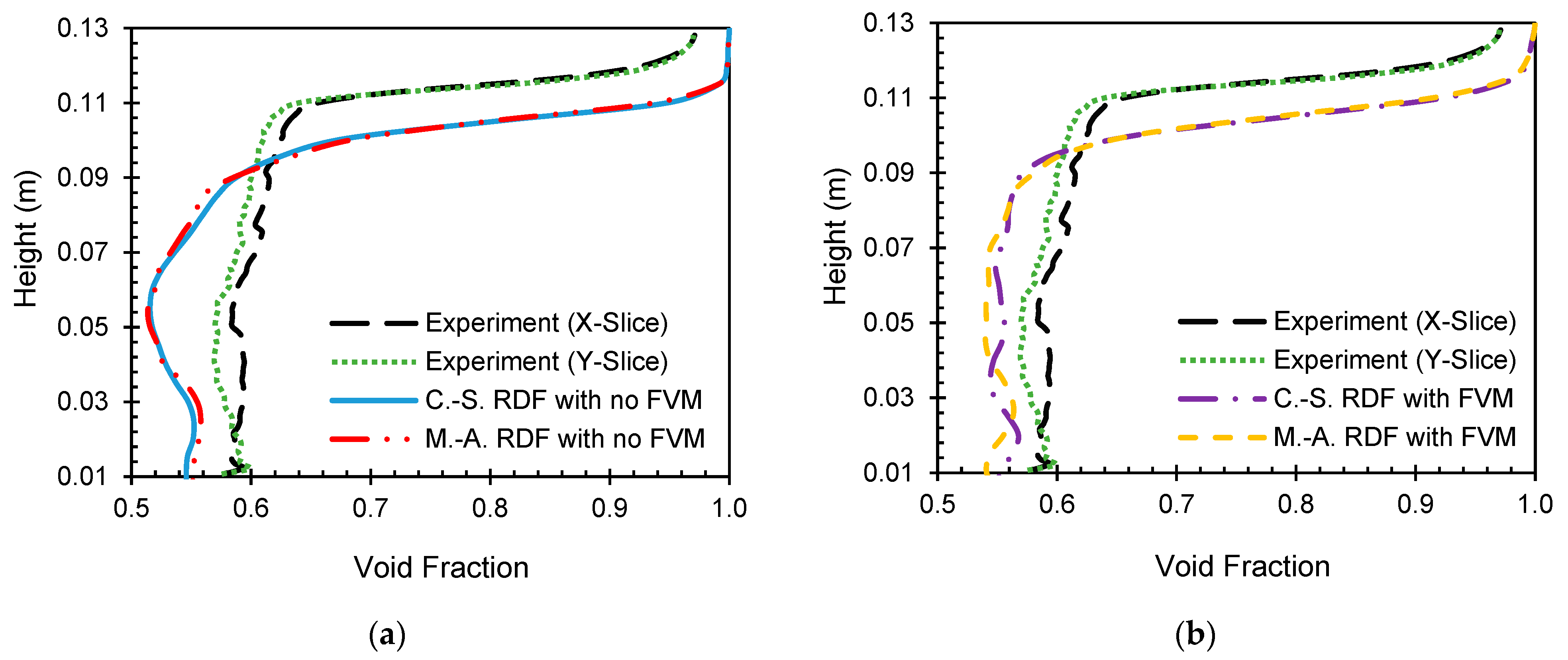
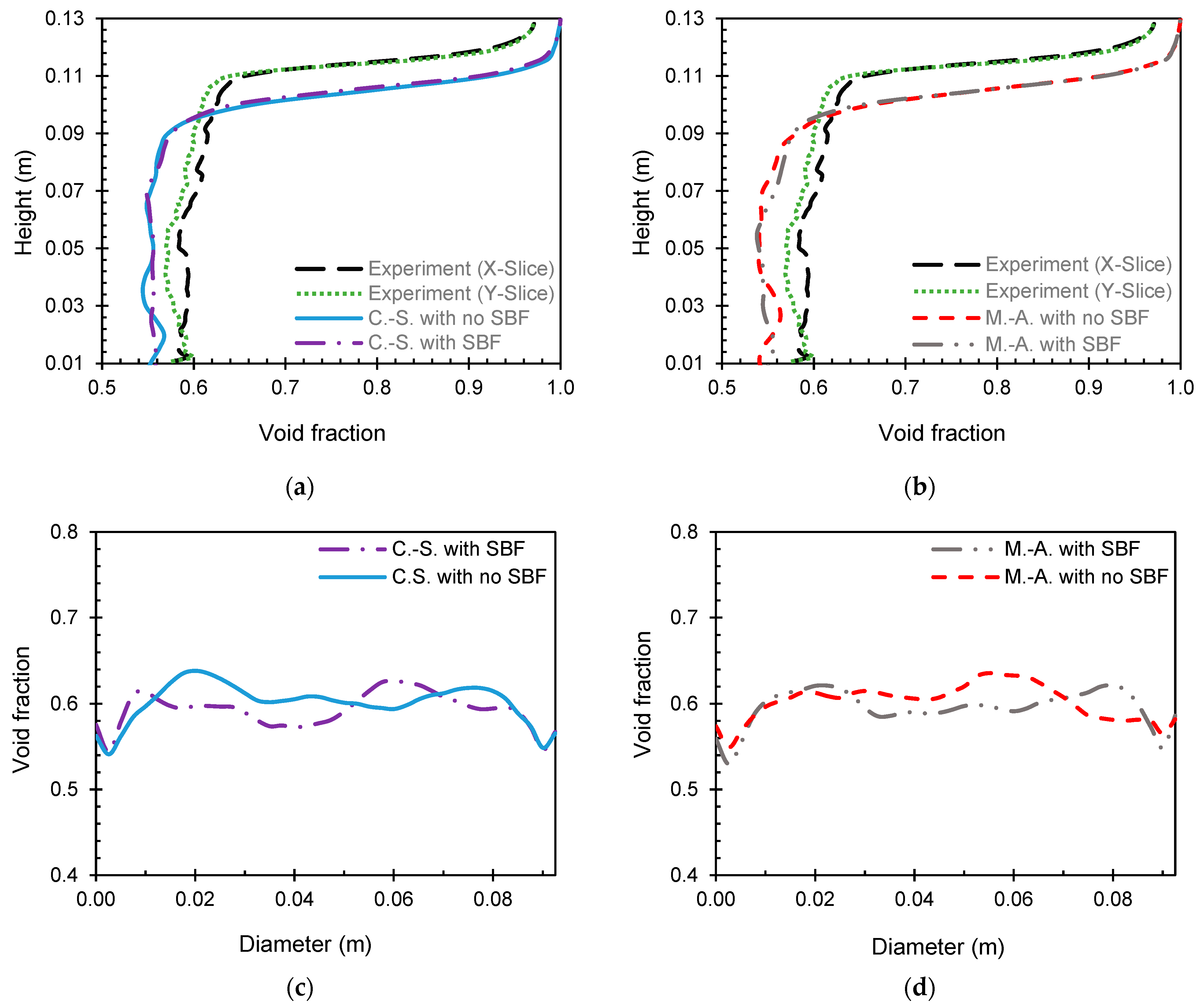
Figure 2 shows the effects of using different RDFs and FVMs on time-averaged void fraction profiles between 2.5 s and 10 s.
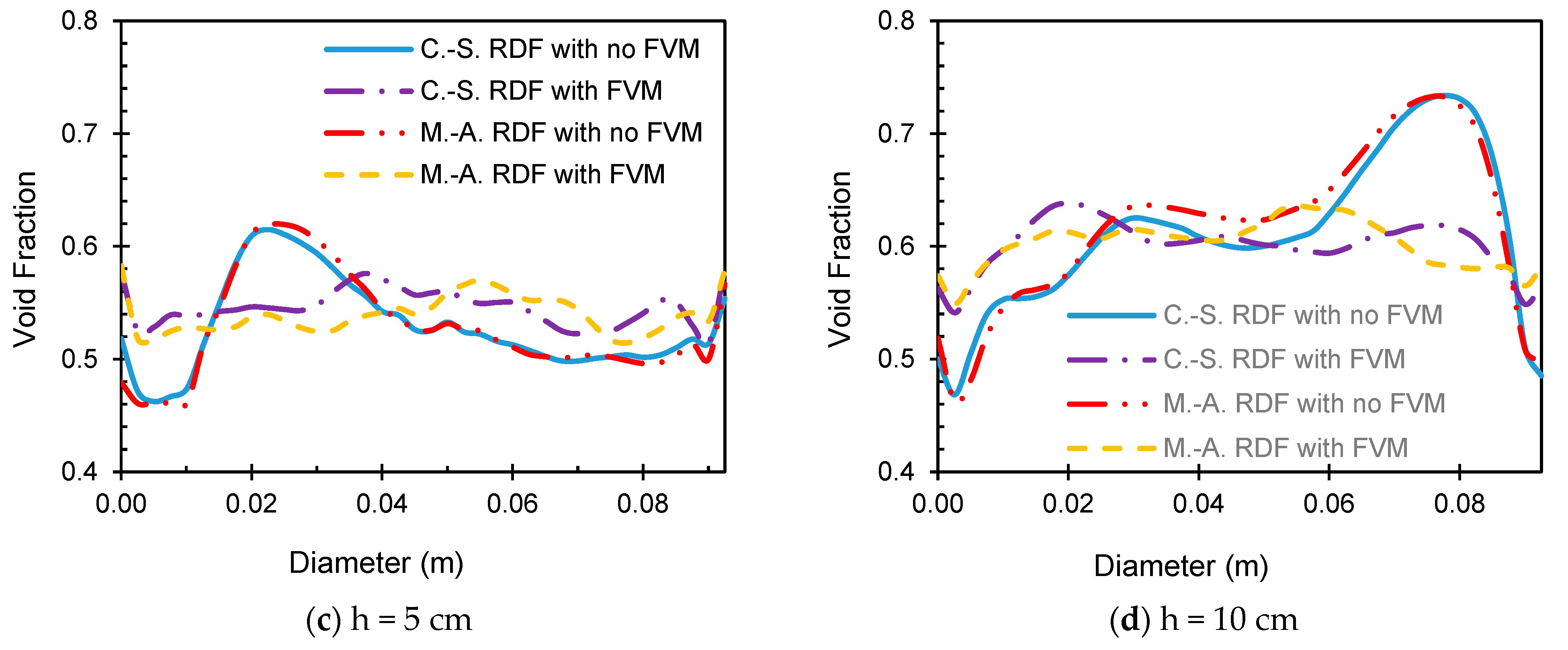
Figure 2a,b present the time-averaged void fraction versus the height of the reactor averaged over the diameter, and
Figure 2c,d illustrate the time-averaged void fraction versus the diameter of the reactor at two different heights of 5cm and 10cm to demonstrate the performance of each combination of models. The experimental data for void fraction were only available against the height of the reactor, which is used to validate simulations in
Figure 2a,b. For the course of this research, the numerical data are time-averaged from 2.5 s to 10 s using an equally spaced time interval of 0.001 s with 7500 time realizations.
Throughout the entire height of the reactor, both RDFs, the Carnahan–Starling and the Ma–Ahmadi, exhibit a more parabolic behavior with no FVM (
Figure 2a), while using the Schaeffer FVM with these RDFs (
Figure 2b) demonstrates more oscillation, which is also characteristic of the experimental data. While the results of all cases are promising, using the Schaeffer model slightly improves the predictions. Despite the slight difference in the void fraction values for these simulations and the experimental data at the same height in the reactor, the use of the Schaeffer FVM aids in predicting the flow more effectively, with the characteristic void fraction oscillation along the height of the fluidized bed before smoothing out toward the value of one in the freeboard. For all simulation cases, the bed height predictions are in agreement with experimental data, where the predicted bed height in all cases is about 1cm lower than the experimental bed height. The effects of using FVM on time-averaged void fraction versus the diameter of the reactor (
Figure 2c,d) is also evident. Although the use of the Schaeffer FVM alters the void fraction predictions, both RDFs show consistent behavior across the diameter of the reactor. The predictions using FVM are smoother at both heights, implying the reactor is predicted to be more stable. As height increases from 5 cm to 10 cm, the range of the void fraction changes increases, which is expected considering the fluidization regime.
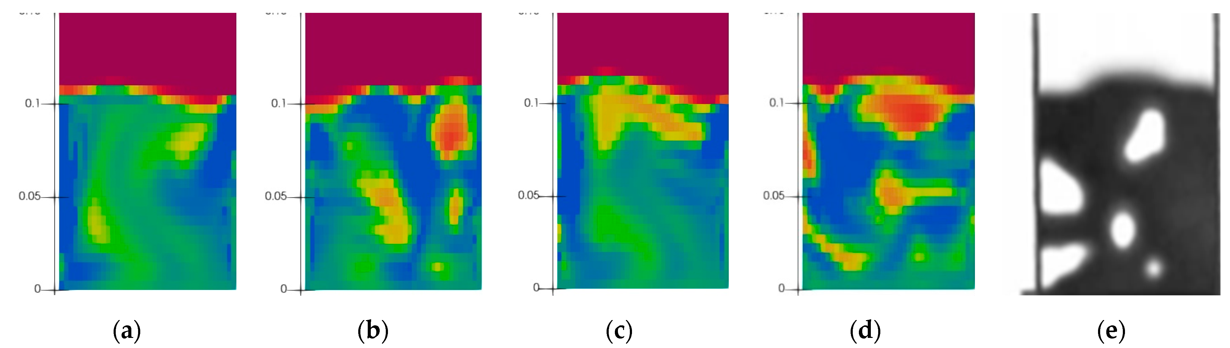
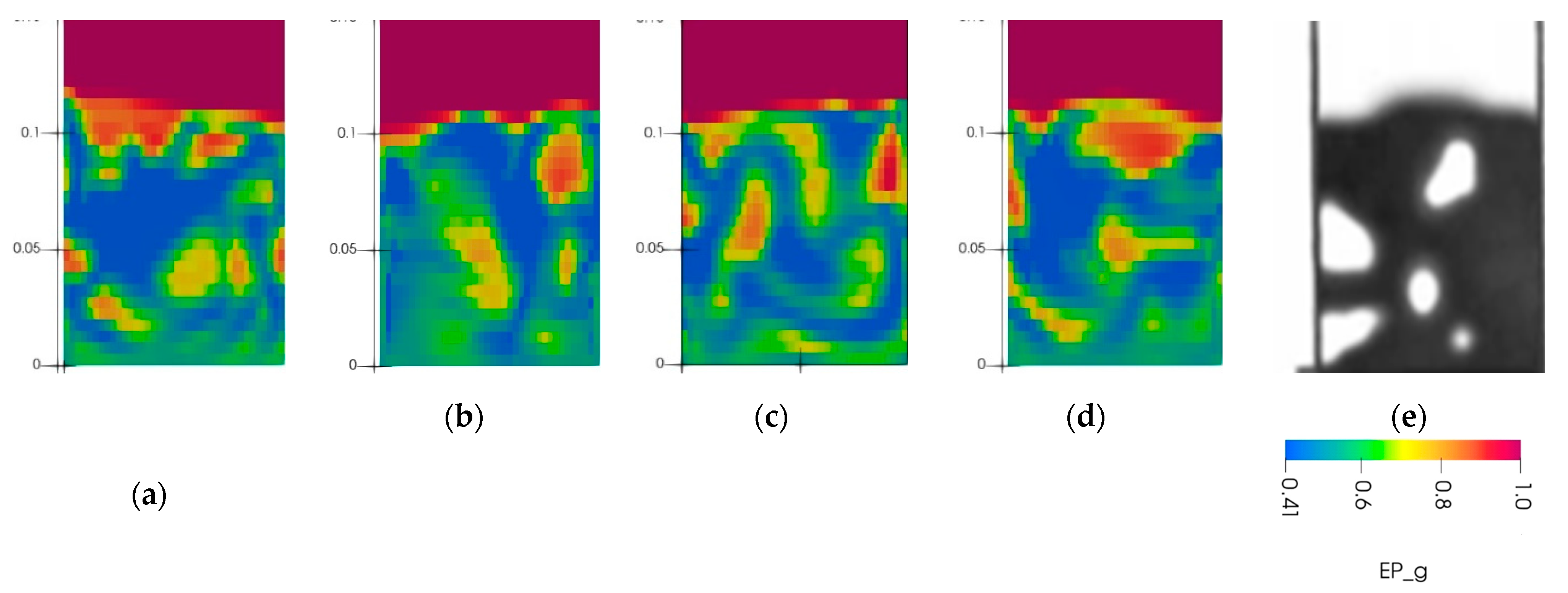
To further analyze the effects of using different models on the behavior of the flow, the instantaneous void fraction contours at 10s for all four cases are presented in
Figure 3. To determine the efficacy of these models, both the Carnahan–Starling and the Ma–Ahmadi RDF with and without the Schaeffer function are compared with the experimental X-Ray of the fluidized bed flow extracted from Deza et al. [
5]. Looking at the experimental X-Ray of the bed, it is evident that the bed contains multiple bubbles. Simulation contours reveal that both RDFs, with the addition of the Schaeffer FVM properly account for the bubbling; however, the number and size of bubbles is better captured using the Ma–Ahmadi RDF. It is also worth mentioning that using the Carnahan–Starling RDF with no FVM shows no signs of any bubbling. However, the use of the Ma–Ahmadi with no FVM predicts the onset of some bubbles. Accordingly, the use of FVM is only recommended for overly packed beds to account for the higher friction level between solid particles. Considering the initial void fraction in this study, the simulated beds are not initially overly packed, which illustrates that the use of FVM is still favorable for beds with low solid concentrations.
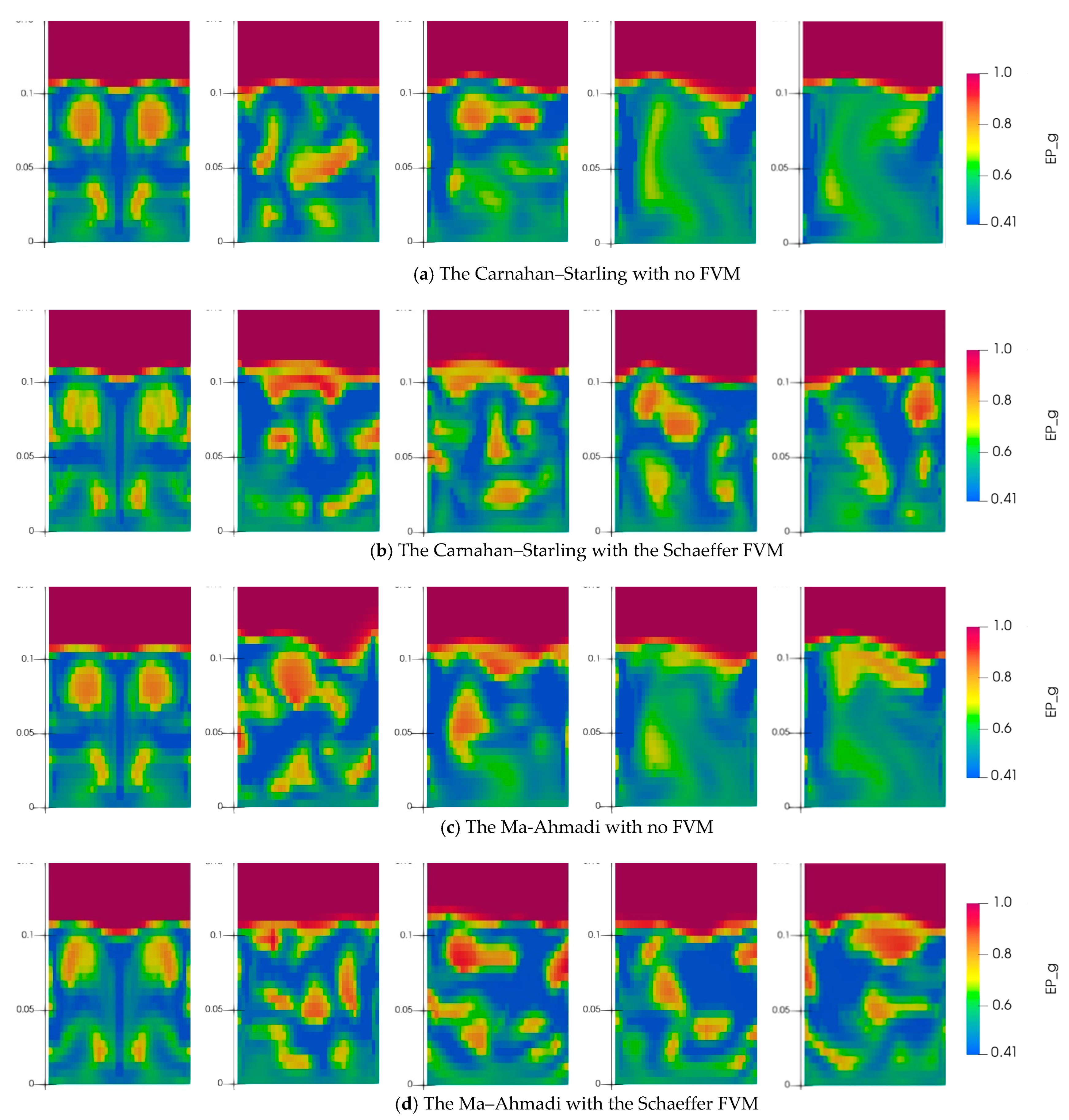
The void fraction contours at multiple timepoints for various combinations of models are presented in
Figure 4. The study of these contours demonstrates the advancement of flow and the bubbling within the flow with time. For all the model combinations, by the time of 1 second from the beginning of the process, the flow has already fluidized.
In the cases with no FVM, some bubbles are present at early times in the flow; however, all bubbles completely disappear by 7.5 seconds. This could be due to the change of the initially uniform solid concentration in different regions of the bed, as initial bubbles form. These changes, consequently, affect particle distances from one another and can create clumps of particles, which potentially affect friction between particles. For the cases with the Schaeffer FVM, bubbles are present throughout the entire flow during the whole time of simulations, which mimics the experimental results. A qualitative comparison between the predictions of the two RDFs accompanying the Schaeffer FVM (
Figure 4b,d) reveals that the Ma–Ahmadi RDF predicts more bubbles during the simulation, which is comparable to the experimental data reported by Deza et al. [
5] shown in
Figure 3e. No significant difference in the size of bubbles is detectable.
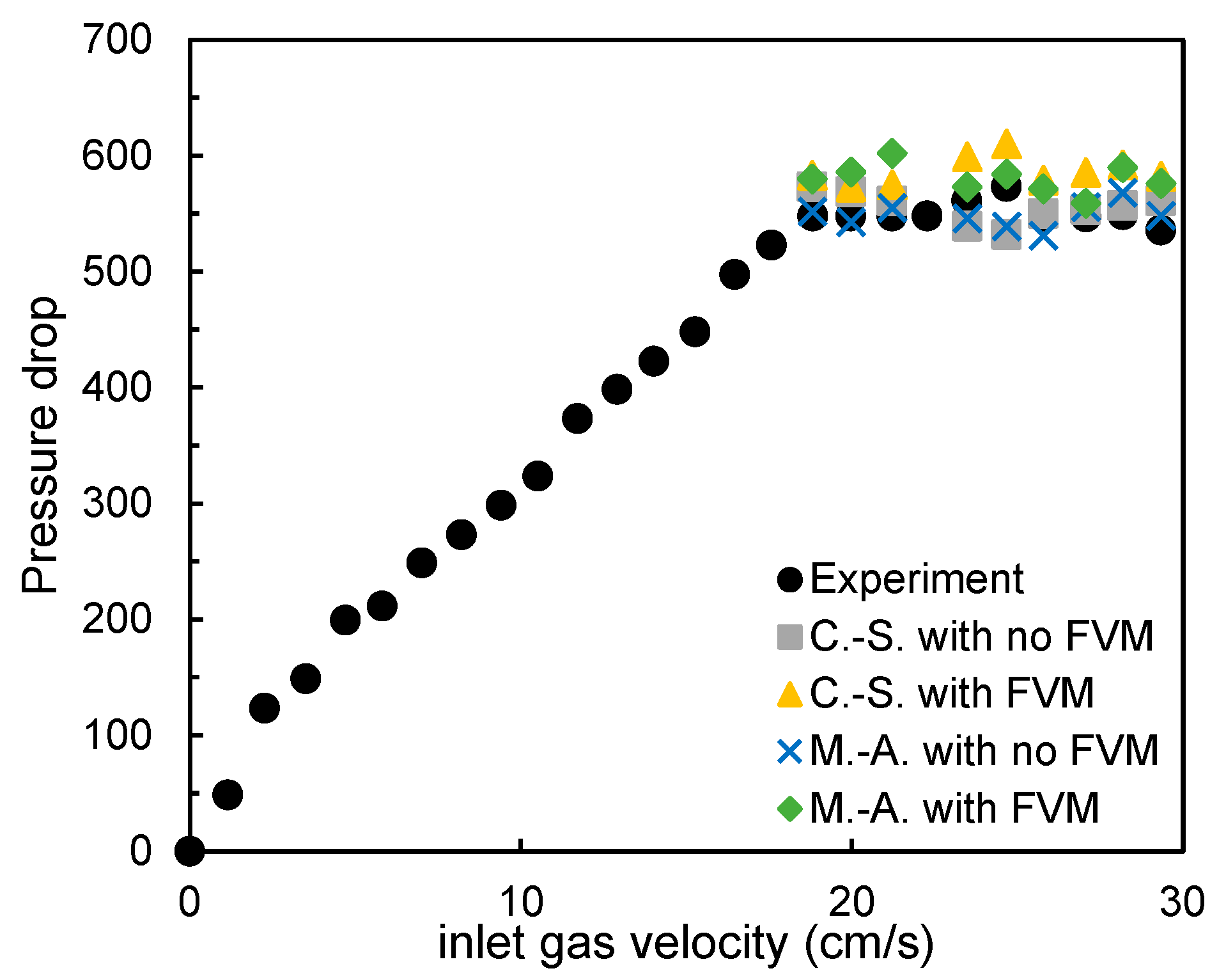
3.1.2. Effects of RDFs and FVMs on Pressure Drop
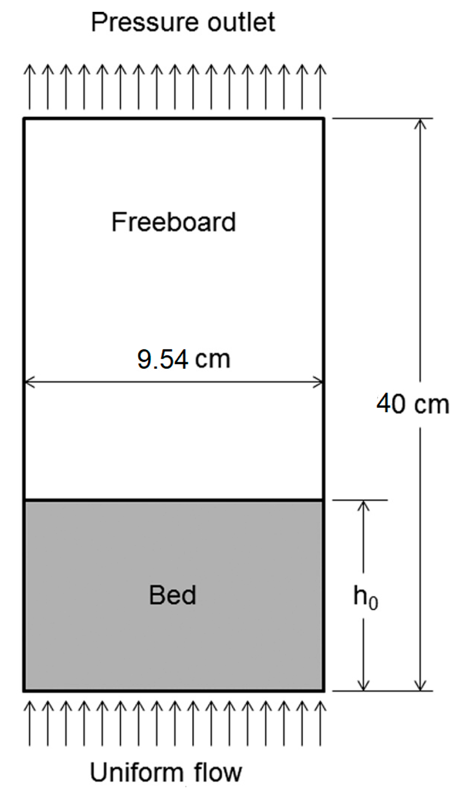
To further investigate the effects of using different RDFs and the effects of applying Schaeffer FVM, pressure drop across the bed is investigated. For Geldart B particles, as the inlet gas velocity increases, the pressure drop across the bed increases linearly until the gas inlet velocity reaches the
and the bed is fully fluidized. In the fully fluidized region, the pressure drop remains constant. At the inlet gas velocity,
, of 24.3 cm/s, which is the
for the rest of this work, the bed is fully fluidized and the fluidization experiments [
5] predicted the pressure drop across the bed to be equal to 570 Pa. At the same velocity, simulations predict a very close pressure drop regardless of the utilized models, where the deviation of simulations from experiments is trivial (less than 2%). To further investigate the behavior of models,
Figure 5 presents the predicted pressure drops by simulations compared to the experimental results at different
’s. For all
’s, the simulation predictions are in good agreement with experiments. The averaged experimental pressure drop in the fully fluidized region is 551 Pa where the value is 555 Pa and 549 Pa for the Carnahan–Staling and the Ma–Ahmadi RDFs with no FVM, respectively. The error associated with both RDFs is less than 1%. However, the utilization of the Schaeffer FVM increases the error associated with the simulations. The averaged pressure drop is 586 Pa and 580 Pa when employing the Carnahan–Starling and the Ma–Ahmadi RDFs with the Schaeffer FVM, respectively. The error associated with the former is 6.5% and the latter is 5%.
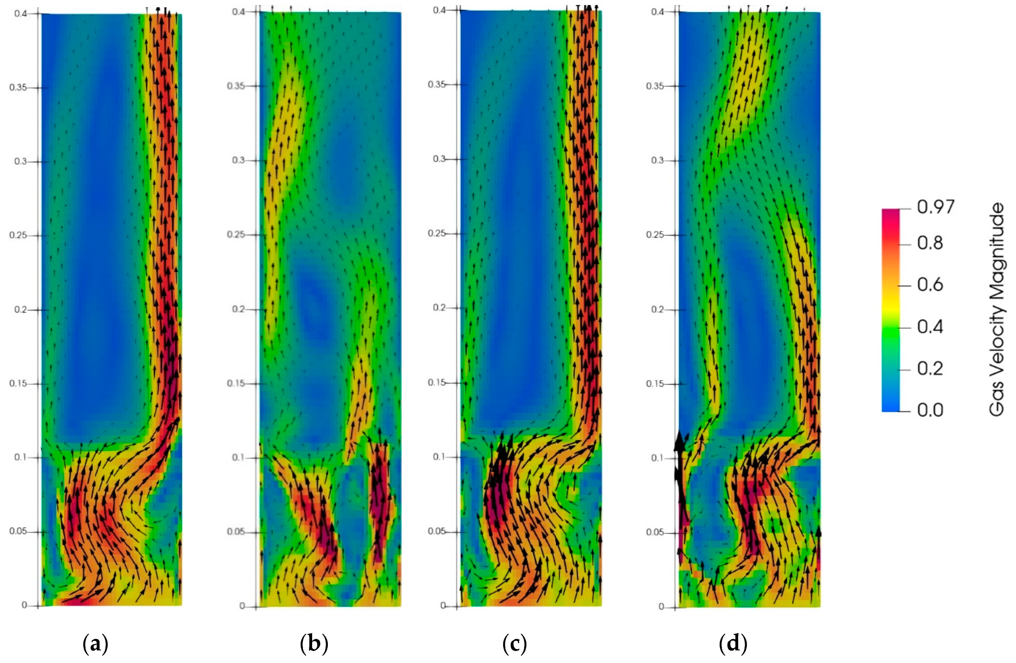
3.1.3. Effects of RDFs and FVMs on Velocity
The dynamics of the flow can be estimated by investigating the gas and solid velocity contours.
Figure 6 and
Figure 7, respectively, contain the gas and solid particle velocity magnitude contours along with the velocity vector at 10 s to better demonstrate the hydrodynamics of the fluidized bed. The use of RDFs with no FVM (
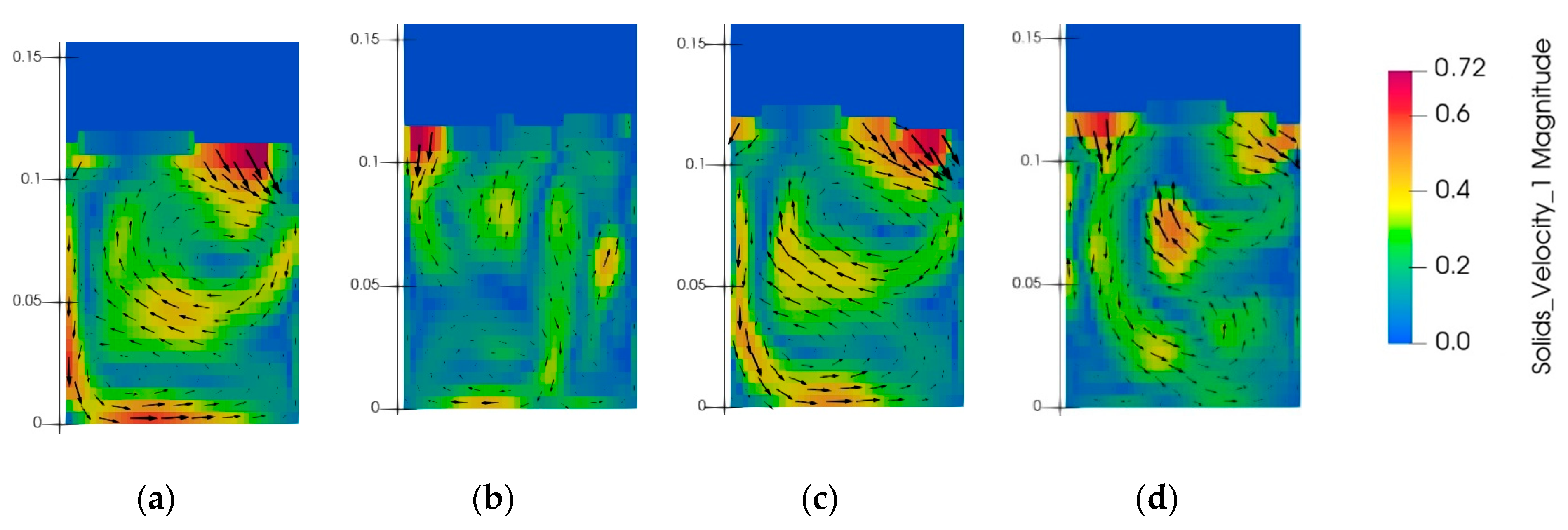
Figure 6a,c) predict similar gas flow, where gas velocity is higher near the center of the reactor close to the left wall in the bed and veers toward the right wall in the freeboard region all the way to the top of the reactor, where gas would leave the reactor. Similarly, predictions of solid velocity for both RDFs (
Figure 7a,c) exhibit similar patterns, where solid particles experience high velocities near the center of the reactor in the vicinity of the left wall. The high velocity regions are also predicted near the left wall, along with the bed entrance and at the right top corner of the bed. The solid velocity vectors show some rotational movement of solid particles where particles are pulled up in the center of the bed and dragged back down into the bed at the right top corner of the reactor where the solid velocity is the highest. This region is where gas flow leaves the bed and leaves the solid particles behind. Although the solid velocity patterns are similar using the two RDFs, the predicted velocity magnitude at different regions are slightly different.
The addition of the Schaeffer FVM (
Figure 6b,d) breaks down the region of higher gas velocities near the center of the bed. The gas flow then oscillates between two walls in the freeboard before leaving the reactor, which varies from the cases without the Schaeffer FVM, which predict a high velocity flow just along the right wall of the reactor (
Figure 6a,c). In spite of the similarities between the predictions of the two RDFs with and without the Schaffer FVM, the predicted gas velocity magnitude is slightly higher using the Ma–Ahmadi RDF. Applying the Schaeffer model also affects the solid velocities (
Figure 7b,d), where higher solid velocities are predicted at some regions near the top of the bed, while within the bed, it predicts pockets of higher solid velocity corresponding to the location between the bubbles in the flow. Although some similarities can be detected between cases with the Schaeffer model (
Figure 7b,d), the predicted solid velocity vectors exhibit different results. The rotational motions are detectable in both cases; however, it is less discernable when using the Carnahan–Starling RDF. The predicted solid velocity magnitude is also lower using this RDF.
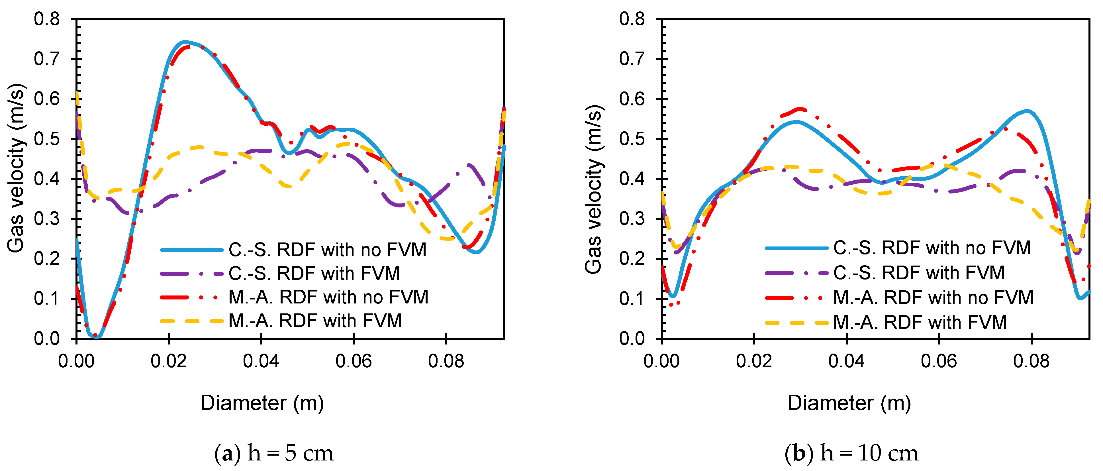
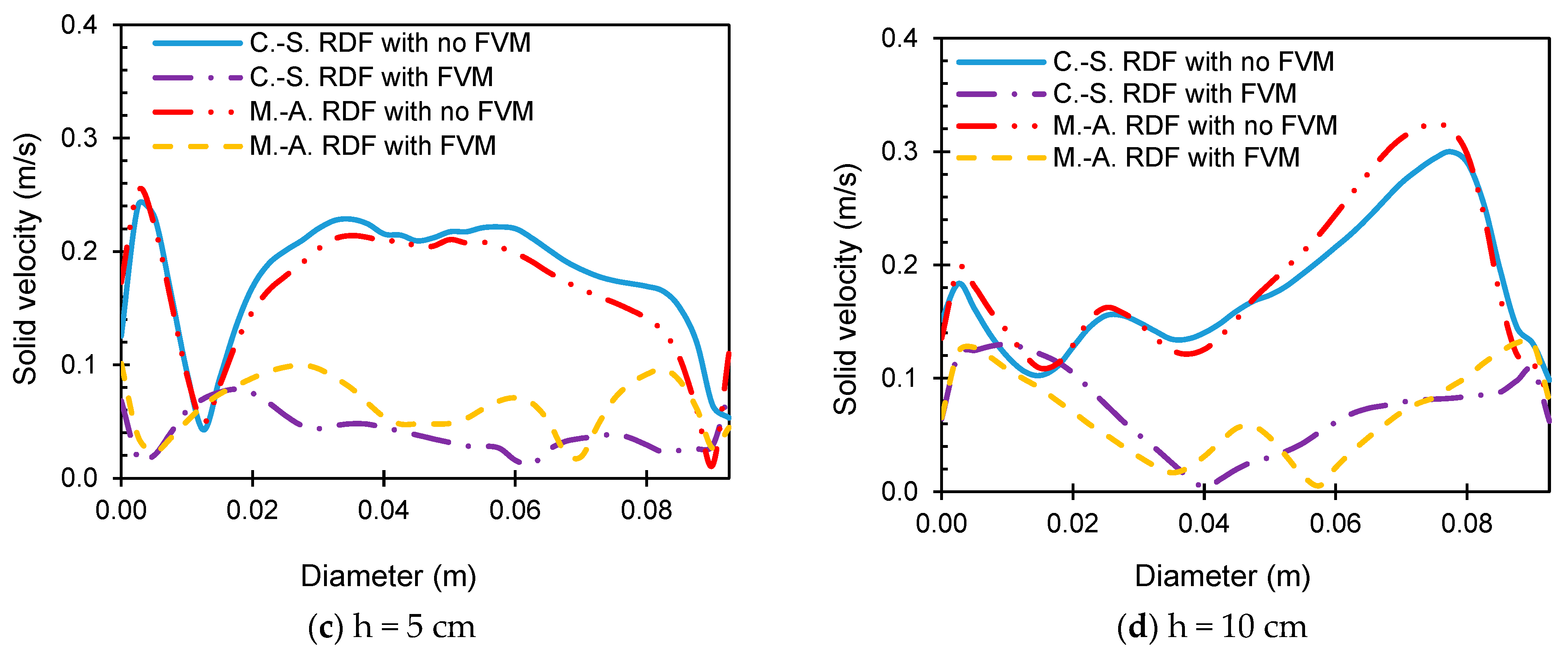
To investigate the effects of using different RDFs and applying FVM more elaborately,
Figure 8 illustrates the time-averaged gas and solid velocity magnitude profiles between 2.5 s and 10 s versus the diameter of the reactor. The profiles are presented in two heights, 5 cm and 10 cm, which are the initial bed heights. Regardless of height, the use of the Schaeffer model predicts significantly lower velocity magnitudes almost everywhere along the diameter of the reactor. This is specifically noticeable in solid velocity magnitude predictions (
Figure 8c,d), where the average solid velocity magnitudes at both heights are about one-third of the predicted value with no FVM. The use of the model also smooths the velocity magnitude predictions at each height, where no significant overshot or undershot of velocity is predicted. At the lower height (h = 5 cm), the range of predicted gas velocity magnitudes are higher for all models compared to h = 10 cm. This can be attributed to the loss of gas momentum, as gas flows higher through the granular bed of materials.
3.2. Effects of
Biomass particles are irregular in shape, and to consider the effects of these irregularities, sphericity is defined and applied to the particle diameter, which results in modeling smaller spherical particles. Considering that particle size has a significant impact on the transitioning between viscous and plastic regimes in a granular system, applying sphericity can change the behavior of the fluidization process. Hence, the value of
that dictates the transfer between viscous and plastic regimes can be affected by particle size. To better understand the effects of
on the simulation predictions, four values of
are tested and the results of these simulations are compared with experimental data [
5]. The variation in
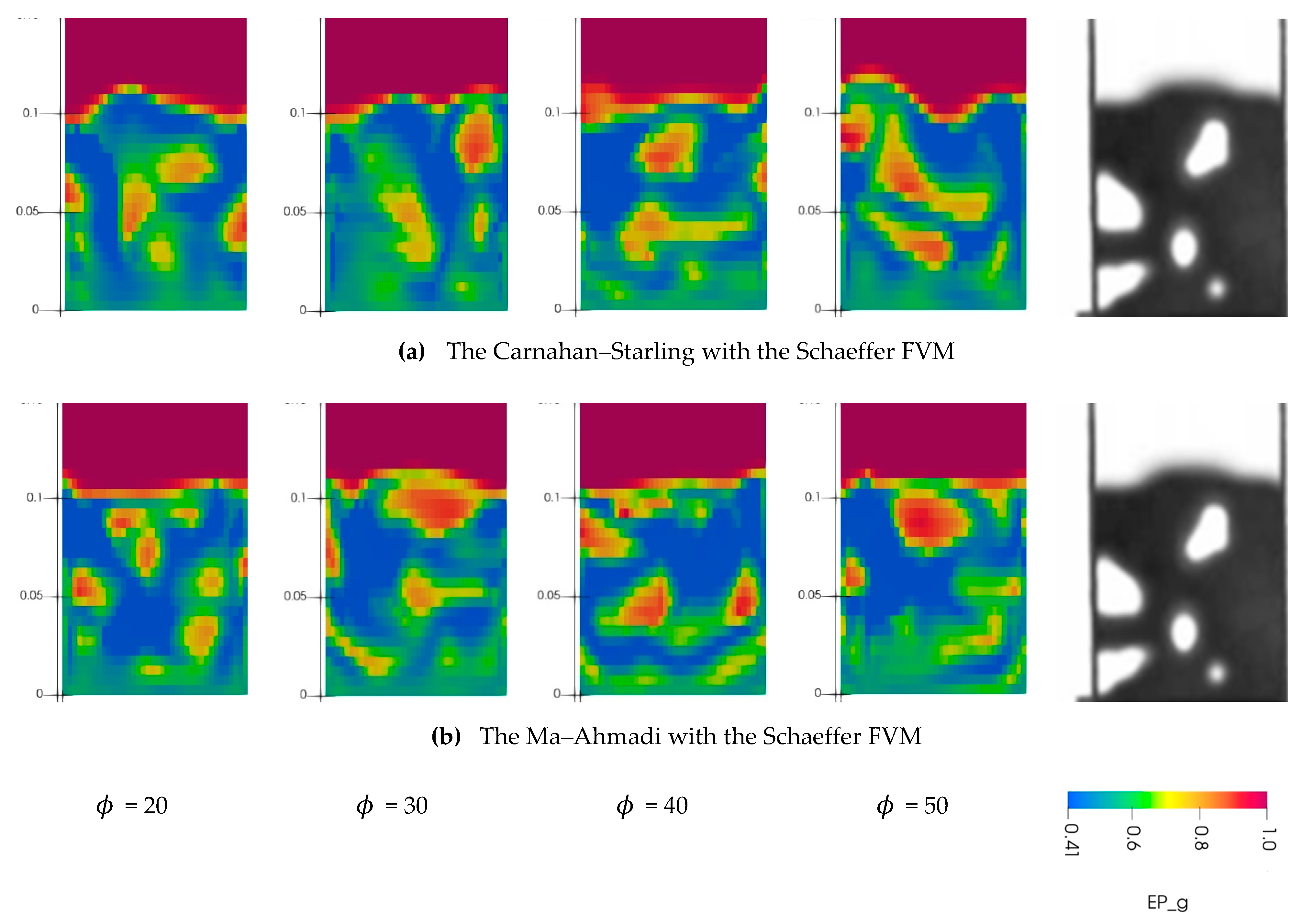
is visualized in
Figure 9 through the void fraction contour plots at 10 s for both RDFs for
between 20 and 50, in increments of ten. These changes were only reported for the cases using the Schaeffer model due to the efficacy of the simulation results of the Schaeffer cases reported previously. The experimental data for void fraction were only available against the height of the reactor, which is used to validate simulations in
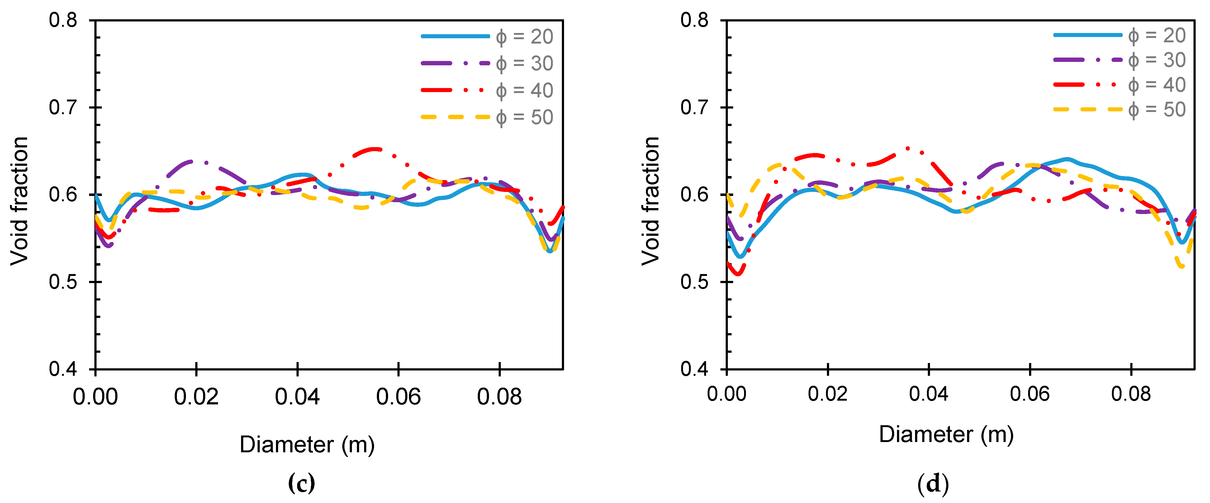
Figure 9a,b.
Figure 9 qualitatively illustrates that increasing the value of
enlarges the size of the bubbles. For
= 20, the bubbles are small and dispersed, while for
= 50, the smaller bubbles merge together and form larger bubbles. Considering that none of these two behaviors are the characteristic of the experimental X-Ray of the bed, the intermediate values of
of 30 and 40 seem to provide the best results in comparison, where the bubbling within the flow is similar to that of the experimental bed. Regardless of the value of
, bubbling behavior predictions of the bed slightly favor the use of the Ma–Ahmadi RDF.
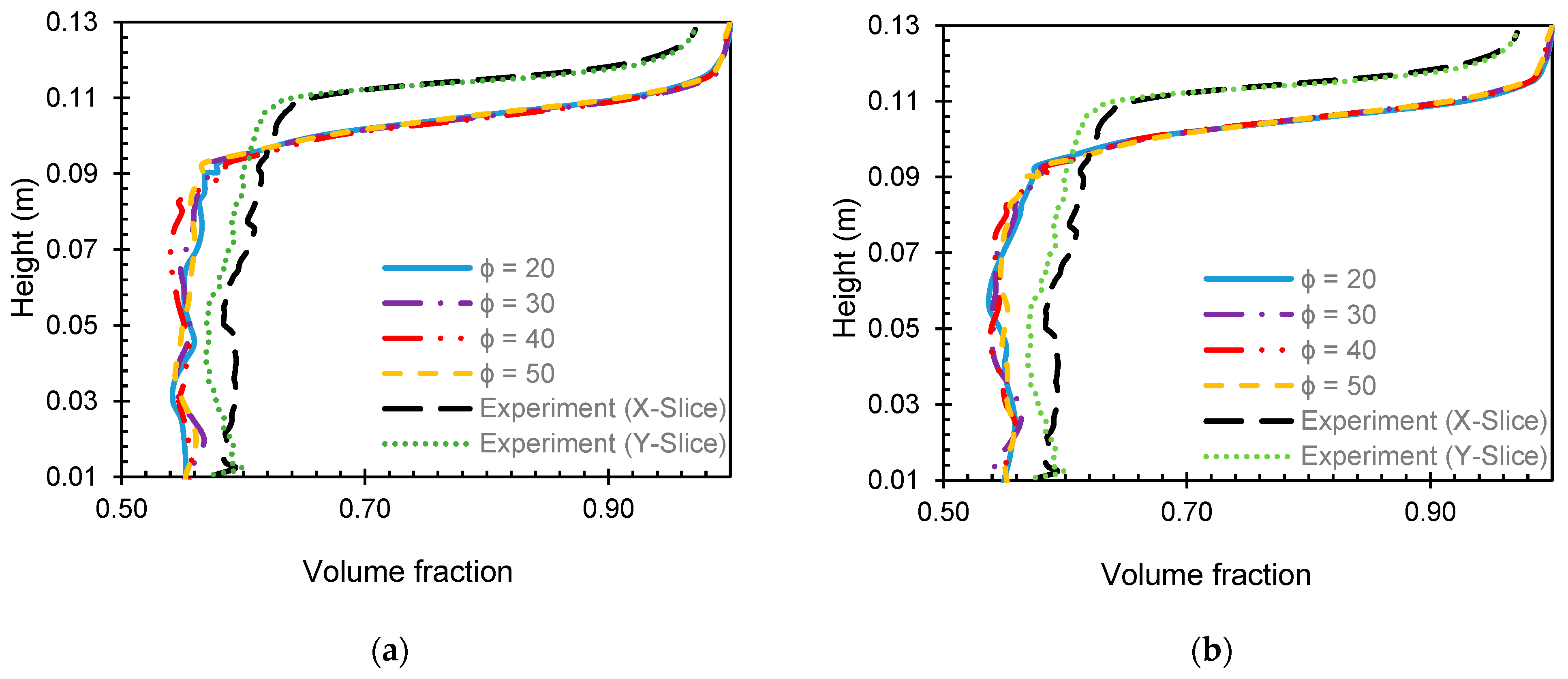
For both RDFs,
Figure 10 presents the time-averaged void fraction profiles between 2.5 s and 10 s versus the height of the reactor averaged over the diameter (
Figure 10a,b) and versus the diameter of the reactor at h = 10 cm (
Figure 10c,d). The plots of the averaged void fraction versus height are compared to the experimental data. In spite of the effects of
on the bubbling behavior of the fluidized bed,
Figure 10 shows no significant effect of
on the time-averaged value of the void fraction. In general, no significant trend and no differences are detected in these results.
3.3. Effects of SBF
The effects of the hyperbolic tangent (tanh) SBF is investigated to determine the efficacy of including the function in future fluidization simulations. The SBF is a smoothing function used to transfer and blend the results between plastic and viscous regions within the fluidized flow. The effects of including the tanh SBF on the instantaneous void fraction contours at 10 s are shown below in
Figure 11. For all simulations performed in this section, the Schaeffer FVM is employed and
was 30 to be able to compare the effects of the smoothing function on previous simulations that were deemed the most successful. A qualitative investigation of the instantaneous void fraction contours reveals that employing the tanh SBF increases the number of bubbles while decreasing the size of the bubbles. The Ma–Ahmadi RDF in combination with the tanh SBF, as compared to the Carnahan–Starling RDF, was a better predictor of the bubbling behavior when compared to experimental results.
Using the same cases, the results are visualized in
Figure 12, using time-averaged plots of void fraction values between 2.5 s and 10 s presented versus the height and the diameter of the reactor. The void fraction is averaged over the diameter when presented against height (
Figure 12a,b), and presented at the height of 10 cm from the reactor inlet, while presented against the diameter of the reactor (
Figure 12c,d). The plots of the averaged void fraction versus height are compared to the experimental data that were available. These plots are less oscillatory in the main area of the bed, making the curve appear flatter when using tanh SBF, particularly at lower heights (up to ~h = 4 cm). The void fraction versus diameter plots does not show any discernible differences with this addition, displaying the same oscillatory behavior as in the previous plots with no SBF. For all plots, the general void fraction values hold true between the plots with and without the addition of the SBF.


