

On the Summarization of Meteorological Data for Solar Thermal Power Generation Forecast


Abstract
:1. Introduction
2. Methodology
2.1. Sandia Selection and Proposed Adoptations
- The cumulative distribution function (CDF) of the meteorological characteristic under evaluation, e.g., temperature, of each candidate (month) is compared to the CDF of the respective months of the long-term meteorological data set. The Finkelstein–Schafer (FS) statistic [31] definition, Equation (1), is used to perform the CDF comparison.
- 2.
- The candidates are ranked according to its FS-statistic, the lower the better, and the top five candidates are selected to the next step;
- 3.
- The top five candidates are evaluated in terms of frequency and length of “runs”, i.e., values for the meteorological characteristic under evaluation over (67th percentile) or below (33rd percentile) the expected range of values. This persistence test excludes the candidate (month) with the longest run (more consecutive days with meteorological characteristic out of expected values), the candidate with the most runs, and a possible candidate with zero runs;
- 4.
- For the remaining candidates, the hourly meteorological characteristic is compared to the hourly average value of the equivalent month from the long-term data set () using the weighted normalized root mean square difference (nRMSD), Equation (3). This slight adaptation of the Sandia method is used to improve the hourly matching of different meteorological characteristics. Pissimanis et al. [32] proposed this step as a replacement for the persistence test (Step 3); here, it is used to increase selection rigor. The normalization is applied by dividing each RMSD for the jth meteorological characteristic by the long-term average, Equation (4);
- 5.
- The twelve selected months are concatenated to compose the TMY.
2.2. Adaptations to Obtain a Typical Meteorological Day
2.3. Performance Metrics
3. Case Studies
4. Results and Discussion
5. Conclusions
Author Contributions
Funding
Data Availability Statement
Acknowledgments
Conflicts of Interest
References
- Mavi, N.K.; Mavi, R.K. Energy and Environmental Efficiency of OECD Countries in the Context of the Circular Economy: Common Weight Analysis for Malmquist Productivity Index. J. Environ. Manag. 2019, 247, 651–661. [Google Scholar] [CrossRef] [PubMed]
- Chen, C.; Pinar, M.; Stengos, T. Renewable Energy Consumption and Economic Growth Nexus: Evidence from a Threshold Model. Energy Policy 2020, 139, 111295. [Google Scholar] [CrossRef]
- IEA. Renewables 2022: Analysis and Forecast to 2027; International Energy Agency: Paris, France, 2022. [Google Scholar]
- Farges, O.; Bézian, J.J.; El Hafi, M. Global Optimization of Solar Power Tower Systems Using a Monte Carlo Algorithm: Application to a Redesign of the PS10 Solar Thermal Power Plant. Renew Energy 2018, 119, 345–353. [Google Scholar] [CrossRef] [Green Version]
- Li, H.; Yang, Y.; Lv, K.; Liu, J.; Yang, L. Compare Several Methods of Select Typical Meteorological Year for Building Energy Simulation in China. Energy 2020, 209, 118465. [Google Scholar] [CrossRef]
- Fan, X.; Chen, B.; Fu, C.; Li, L. Research on the Influence of Abrupt Climate Changes on the Analysis of Typical Meteorological Year in China. Energies 2020, 13, 6531. [Google Scholar] [CrossRef]
- Hall, I.J.; Prairie, R.R.; Anderson, H.E.; Boes, E.C. Generation of a Typical Meteorological Year; Sandia Labs.: Albuquerque, NM, USA, 1978. [Google Scholar]
- Andersen, B.; Eidorff, S.; Lund, H.; Pedersen, E.; Rosenørn, S.; Valbjørn, O. General Rights Meteorological Data for Design of Building and Installation: Meteorological Data for Design of Building and Installation; Statens Byggeforskning Institut: Hørsholm, Denmark, 1977. [Google Scholar]
- Crow, L.W. Weather Year for Energy Calculations. ASHRAE J. 1984, 26, 42–47. [Google Scholar]
- Gazela, M.; Mathioulakis, E. A New Method for Typical Weather Data Selection to Evaluate Long-Term Performance of Solar Energy Systems. Sol. Energy 2001, 70, 339–348. [Google Scholar] [CrossRef]
- Kambezidis, H.D.; Psiloglou, B.E.; Kaskaoutis, D.G.; Karagiannis, D.; Petrinoli, K.; Gavriil, A.; Kavadias, K. Generation of Typical Meteorological Years for 33 Locations in Greece: Adaptation to the Needs of Various Applications. Theor. Appl. Climatol. 2020, 141, 1313–1330. [Google Scholar] [CrossRef]
- Zang, H.; Wang, M.; Huang, J.; Wei, Z.; Sun, G. A Hybrid Method for Generation of Typical Meteorological Years for Different Climates of China. Energies 2016, 9, 1094. [Google Scholar] [CrossRef] [Green Version]
- Amega, K.; Laré, Y.; Moumouni, Y.; Bhandari, R.; Madougou, S. Development of Typical Meteorological Year for Massive Renewable Energy Deployment in Togo. Int. J. Sustain. Energy 2022, 41, 1739–1758. [Google Scholar] [CrossRef]
- Bre, F.; Fachinotti, V.D. Generation of Typical Meteorological Years for the Argentine Littoral Region. Energy Build 2016, 129, 432–444. [Google Scholar] [CrossRef]
- Dorneles, R.; Bravo, G.; Starke, A.; Lemos, L.; Colle, S. Generation of 441 Typical Meteorological Year from Inmet Stations—Brazil. In Proceedings of the ISES Solar World Congress 2019, Santiago, Chile, 4–7 November 2019; International Solar Energy Society: Freiburg, Germany, 2019; pp. 1–12. [Google Scholar]
- Chan, A.L.S. Generation of Typical Meteorological Years Using Genetic Algorithm for Different Energy Systems. Renew Energy 2016, 90, 1–13. [Google Scholar] [CrossRef]
- Kumar, D.S.; Yagli, G.M.; Kashyap, M.; Srinivasan, D. Solar Irradiance Resource and Forecasting: A Comprehensive Review. IET Renew. Power Gener. 2020, 14, 1641–1656. [Google Scholar] [CrossRef]
- Yang, B.; Zhu, T.; Cao, P.; Guo, Z.; Zeng, C.; Li, D.; Chen, Y.; Ye, H.; Shao, R.; Shu, H.; et al. Classification and Summarization of Solar Irradiance and Power Forecasting Methods: A Thorough Review. CSEE J. Power Energy Syst. 2021. [Google Scholar] [CrossRef]
- Yang, B.; Zhu, T.; Cao, P.; Guo, Z.; Zeng, C.; Li, D.; Chen, Y.; Ye, H.; Shao, R.; Shu, H.; et al. Calculating the Financial Value of a Concentrated Solar Thermal Plant Operated Using Direct Normal Irradiance Forecasts. Sol. Energy 2016, 125, 267–281. [Google Scholar] [CrossRef] [Green Version]
- Luo, X.; Zhang, D. An Adaptive Deep Learning Framework for Day-Ahead Forecasting of Photovoltaic Power Generation. Sustain. Energy Technol. Assess. 2022, 52, 102326. [Google Scholar] [CrossRef]
- Rana, M.; Sethuvenkatraman, S.; Heidari, R.; Hands, S. Solar Thermal Generation Forecast via Deep Learning and Application to Buildings Cooling System Control. Renew Energy 2022, 196, 694–706. [Google Scholar] [CrossRef]
- Dobos, A.; Gilman, P.; Kasberg, M. P50/P90 Analysis for Solar Energy Systems Using the System Advisor Model. In Proceedings of the 2012 World Renewable Energy Forum, Denver, CO, USA, 13–17 May 2012. [Google Scholar]
- Vasallo, M.J.; Bravo, J.M. A Novel Two-Model Based Approach for Optimal Scheduling in CSP Plants. Sol. Energy 2016, 126, 73–92. [Google Scholar] [CrossRef]
- Monjurul Ehsan, M.; Guan, Z.; Gurgenci, H.; Klimenko, A. Novel Design Measures for Optimizing the Yearlong Performance of a Concentrating Solar Thermal Power Plant Using Thermal Storage and a Dry-Cooled Supercritical CO2 Power Block. Energy Convers. Manag. 2020, 216, 112980. [Google Scholar] [CrossRef]
- Brodrick, P.G.; Kang, C.A.; Brandt, A.R.; Durlofsky, L.J. Optimization of Carbon-Capture-Enabled Coal-Gas-Solar Power Generation. Energy 2015, 79, 149–162. [Google Scholar] [CrossRef]
- NREL NSRDB Data Viewer. Available online: https://maps.nrel.gov/nsrdb-viewer (accessed on 6 November 2020).
- Orsini, R.M.; Brodrick, P.G.; Brandt, A.R.; Durlofsky, L.J. Computational Optimization of Solar Thermal Generation with Energy Storage. Sustain. Energy Technol. Assess. 2021, 47, 101342. [Google Scholar] [CrossRef]
- National Renewable Energy Laboratory. User’s Manual National Solar Radiation Data Base (NSRDB); National Renewable Energy Laboratory: Golden, CO, USA, 1992. [Google Scholar]
- Marion, W.; Urban, K. User’s Manual for TMY2s: Derived from the 1961–1990 National Solar Radiation Data Base; National Renewable Energy Lab.: Golden, CO, USA, 1995. [Google Scholar]
- Wilcox, S.; Marion, W. Users Manual for TMY3 Data Sets (Revised); National Renewable Energy Lab.: Golden, CO, USA, 2008. [Google Scholar]
- Finkelstein, J.M.; Schafer, R.E. Improved Goodness-Of-Fit Tests. Biometrika 1971, 58, 641–645. [Google Scholar] [CrossRef]
- Pissimanis, D.; Karras, G.; Notaridou, V.; Gavra, K. The Generation of a “Typical Meteorological Year” for the City of Athens. Sol. Energy 1988, 40, 405–411. [Google Scholar] [CrossRef]
- Vilasboas, I.F.; dos Santos, V.G.S.F.; de Morais, V.O.B.; Ribeiro, A.S.; da Silva, J.A.M. AERES: Thermodynamic and Economic Optimization Software for Hybrid Solar–Waste Heat Systems. Energies 2022, 15, 4284. [Google Scholar] [CrossRef]


| Characteristic | Weights |
|---|---|
| Mean dry bulb temperature | 2/10 |
| Mean wind velocity | 2/10 |
| Effective direct normal irradiance | 6/10 |
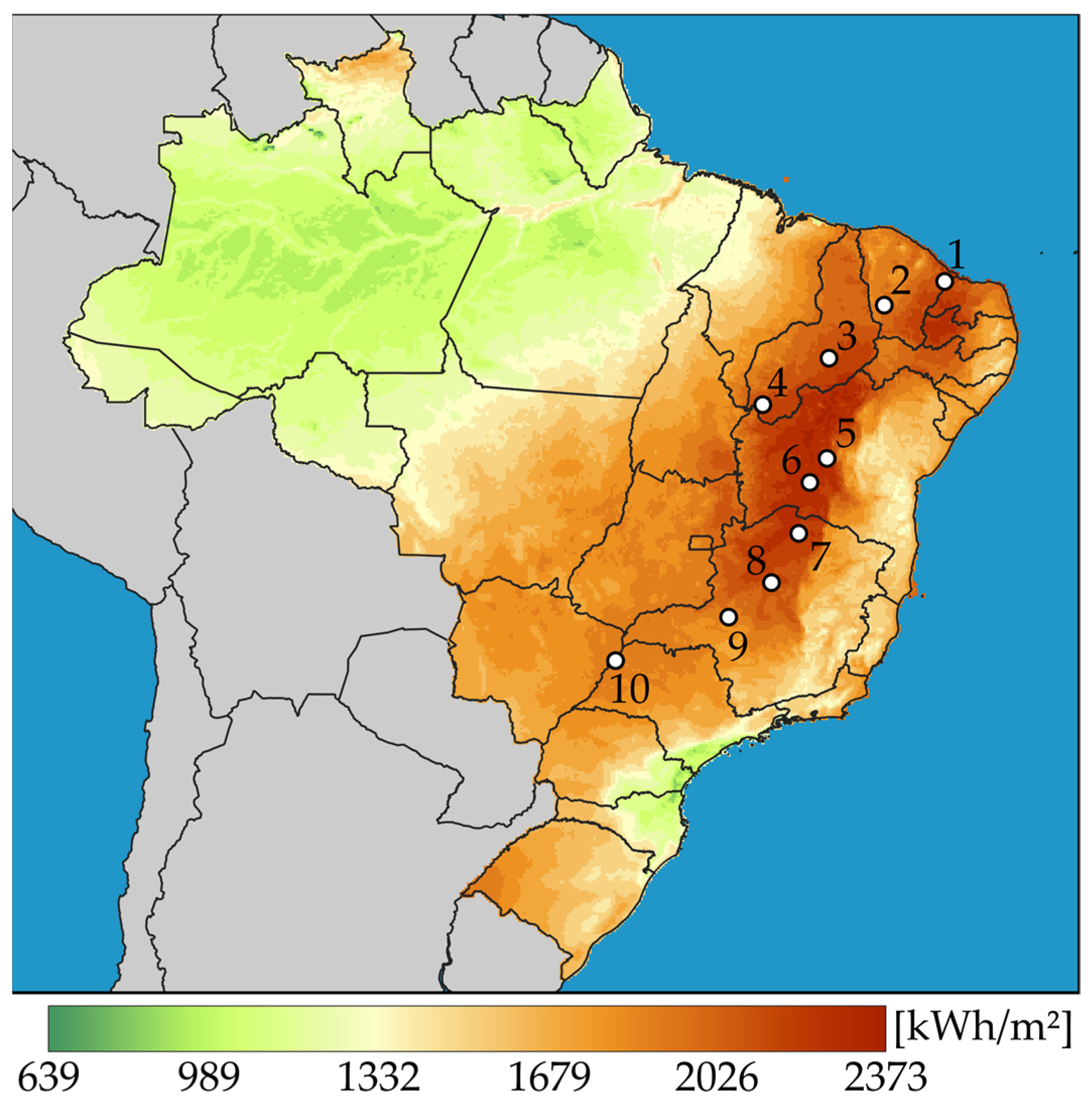
| Id. | City | State | Lat/Lon | Overall Average DNI [W/m²] * | Overall Average Temperature [°C] * | Overall Average Wind Speed [m/s²] * |
|---|---|---|---|---|---|---|
| 1 | Quixeré | CE | −5.03/−37.78 | 553.43 | 27.13 | 4.46 |
| 2 | Tauá | CE | −6.03/−40.26 | 530.51 | 26.01 | 3.28 |
| 3 | Ribeira do Piauí | PI | −8.19/−42.54 | 545.54 | 28.24 | 2.72 |
| 4 | São Gonçalo do Gurguéia | PI | −10.11/−45.26 | 564.14 | 25.11 | 2.26 |
| 5 | Oliveira dos Brejinhos | BA | −12.31/−42.62 | 606.88 | 25.27 | 1.81 |
| 6 | Bom Jesus da Lapa | BA | −13.31/−43.34 | 592.02 | 26.48 | 2.68 |
| 7 | Jaíba | MG | −15.39/−43.78 | 593.11 | 25.35 | 2.20 |
| 8 | Pirapora | MG | −17.43/−44.9 | 571.80 | 23.85 | 2.11 |
| 9 | Guimarânia | MG | −18.83/−46.66 | 526.29 | 21.26 | 2.07 |
| 10 | Pereira Barreto | SP | −20.63/−51.30 | 528.73 | 24.39 | 2.36 |
| System | Component | Details |
|---|---|---|
| Solar field | Parabolic through collectors | Concentrator: SkyFuel SkyTrough; |
| Absorber: Solel UVAC3; | ||
| Aperture area: 234,067 m²; | ||
| Hot temperature: 331.80 °C; | ||
| Cold temperature: 119.11 °C; | ||
| Heat transfer fluid (HFT): Dowtherm A; | ||
| Obs.: without fossil backup. | ||
| Power block | Organic Rankine cycle | Design point: HTF inlet temperature: 331.80 °C; HTF outlet temperature: 119.11 °C; Required mass flow: 74.74 m³/s. |
| Net power: 2749.38 We; | ||
| Efficiency: 8.18%. | ||
| Storage | Direct storage system–two tanks | Storage capacity: 7.55 h; |
| Hot tank temperature: 331.80 °C; | ||
| Cold tank temperature: 119.11 °C; | ||
| Thermal fluid: Dowtherm A; | ||
| Obs.: electrical heater to compensate losses ). |
Disclaimer/Publisher’s Note: The statements, opinions and data contained in all publications are solely those of the individual author(s) and contributor(s) and not of MDPI and/or the editor(s). MDPI and/or the editor(s) disclaim responsibility for any injury to people or property resulting from any ideas, methods, instructions or products referred to in the content. |
© 2023 by the authors. Licensee MDPI, Basel, Switzerland. This article is an open access article distributed under the terms and conditions of the Creative Commons Attribution (CC BY) license (https://creativecommons.org/licenses/by/4.0/).
Share and Cite
Vilasboas, I.F.; da Silva, J.A.M.; Venturini, O.J. On the Summarization of Meteorological Data for Solar Thermal Power Generation Forecast. Energies 2023, 16, 3297. https://doi.org/10.3390/en16073297
Vilasboas IF, da Silva JAM, Venturini OJ. On the Summarization of Meteorological Data for Solar Thermal Power Generation Forecast. Energies. 2023; 16(7):3297. https://doi.org/10.3390/en16073297
Chicago/Turabian StyleVilasboas, Icaro Figueiredo, Julio Augusto Mendes da Silva, and Osvaldo José Venturini. 2023. "On the Summarization of Meteorological Data for Solar Thermal Power Generation Forecast" Energies 16, no. 7: 3297. https://doi.org/10.3390/en16073297
APA StyleVilasboas, I. F., da Silva, J. A. M., & Venturini, O. J. (2023). On the Summarization of Meteorological Data for Solar Thermal Power Generation Forecast. Energies, 16(7), 3297. https://doi.org/10.3390/en16073297