The Economics of Gasification: A Market-Based Approach

Abstract

This paper deals with the economics of gasification facilities in general and IGCC power plants in particular. Regarding the prospects of these systems, passing the technological test is one thing, passing the economic test can be quite another. In this respect, traditional valuations assume constant input and/or output prices. Since this is hardly realistic, we allow for uncertainty in prices. We naturally look at the markets where many of the products involved are regularly traded. Futures markets on commodities are particularly useful for valuing uncertain future cash flows. Thus, revenues and variable costs can be assessed by means of sound financial concepts and actual market data. On the other hand, these complex systems provide a number of flexibility options (e.g., to choose among several inputs, outputs, modes of operation, etc.). Typically, flexibility contributes significantly to the overall value of real assets. Indeed, maximization of the asset value requires the optimal exercise of any flexibility option available. Yet the economic value of flexibility is elusive, the more so under (price) uncertainty. And the right choice of input fuels and/or output products is a main concern for the facility managers. As a particular application, we deal with the valuation of input flexibility. We follow the Real Options approach. In addition to economic variables, we also address technical and environmental issues such as energy efficiency, utility performance characteristics and emissions (note that carbon constraints are looming). Lastly, a brief introduction to some stochastic processes suitable for valuation purposes is provided.

1. Introduction

From an economic point of view, perhaps the best suited description of gasification is the following: “Gasification is a flexible, commercially proven, and efficient technology that produces the building blocks for a range of high-value products from a variety of low-value feedstocks” (Gasification Technologies Council [1]). In view of that, this work focuses on system flexibility issues optimizing inputs and outputs in addition to gasifier designs and processes. As stated at the very start in Trigeorgis [2]: “Flexibility has value”. Assessing its value at the applied level, though, is far from obvious.

Regarding energy investments, first we note the random character of both input and output prices. Second, scientific and technological developments take place continuously in unpredictable ways. Third, the institutional framework within which relevant players operate changes from time to time in response to new circumstances. On the other hand, these investments are at least partially irreversible, i.e., should market conditions turn, the firm cannot “uninvest” and recover the full expenditure. Further, usually the firm has the opportunity (not the obligation) to invest in a project over some pre-specified period of time; i.e., it has to decide whether and when to invest. In the particular case of gasification facilities, this scenario combines with other options to manage the energy project in flexible ways.

Under these circumstances, valuation techniques based on the methods for pricing options (such as Contingent Claims Analysis or Dynamic Programming) are superior to the traditional approaches that are based on discounted cash flows (see, for instance, Dixit and Pindyck [3]; Sick [4]; Trigeorgis [2]). Specific applications to energy investments can be found in Ronn [5], and the Real Options Group web site (http://www.realoptions.org). Now in this paper we address the main elements to be considered in an economic valuation of gasification technologies in general, and Integrated Gasification Combined Cycle (IGCC) power plants in particular. The particular choice between burning coal or natural gas for producing power has been previously analyzed in Abadie and Chamorro [6]. These investments enjoy a long useful life but require some non-negligible time to build. In the medium to long term, their ultimate fate will depend on their economic profitability. In this respect, any economic assessment should take into account both the potential profits and risks inherent to these technologies.

Some of the advantages can be directly measured. Thus, most importantly, gasification technologies allow choosing the cheapest fuel from a range of alternatives. This is in stark contrast to pricier resources for inflexible technologies, such as natural gas-fired combined cycles (NGCC) in power production. Since investments in power generation involve long-lived assets, a proper valuation of this fuel price gap in the future is crucial. Note, though, that there may not be markets for some of the commodities involved in exploiting these technologies, despite the fact that they do have an economic value. For instance, municipal and industrial wastes could be deemed worthless (or even costly to store or treat), but they can be transformed into high-value products. The same can also apply to certain pollutant emissions if a market for them is (still) in the offing. This possibility should not be overlooked.

As mentioned above, not only returns are important but risks as well. Whatever their nature happens to be (financial, operational, regulatory, ...), these risks must be quantified. Needless to say, any measure targeted at reducing them will contribute to the development of this technology. Some major aspects on risk management are highlighted below:

• Risk related to the possibility of more stringent environmental regulations. They could result in a higher operating cost for coal-based technologies as compared with competing low-emission (natural gas) or clean technologies (nuclear, wind, solar). In countries with this kind of regulation in place, future regulatory developments always spell uncertainty and therefore volatility in the emission allowance price.
• Risk related to the identity of the marginal technology in power production. Natural gas-fired plants are usually the marginal technology; as such, they set the market price of electricity according to their short-term marginal costs. In particular, lower carbon emissions from gas plants (relative to coal plants) mean that these plants need less emissions allowances per unit of electricity. Therefore, the price of electricity would partially reflect their lower emissions. In other words, this price would be “unduly low” from coal plants’ perspective. These plants could thus find it difficult to recover some fraction of their costs through the electricity price (the more so if carbon prices rise). One possible reaction would be to retrofit them for capturing carbon.
• Risk related to the development of the gasification technology because of a lack of standards and modularization.

This paper is organized as follows:

• Section 2 introduces gasification processes and technologies; special focus is placed on the flexibilities that are available to the managers.
• Coal, one of several feedstocks suitable for gasification, is briefly addressed in Section 3.
• If we are assessing a potential investment in this technology we need to identify the more relevant issues. Section 4 is devoted to those issues for which markets are particularly worth considering. This clearly holds for primary energy markets. Coal and natural gas prices are regularly determined on futures markets, and the information they convey cannot be overlooked. Of course, identifying the cheapest fuel is important when, from the outset, the plant is restricted to use one single fuel; and, at least in this case, it is also relatively simple. When there is flexibility, though, this important issue becomes more complex. This is because the cheapest fuel can change from time to time and fuel switching costs may be a barrier to seize this opportunity. Next, the market for electricity is relevant from the revenue side. However, (futures) markets for electricity are not as developed as those for oil, coal or natural gas. In spite of this, electricity prices play a crucial role in the economics of a given power station: the merit order influences dispatch of every plant, which in turn affects its availability rate. Moreover, the utilities that operate under environmental restrictions must closely watch emissions markets (for sulfur, carbon, etc.). In addition to variable costs and revenues, construction costs are of paramount importance for the profitability of these capital-intensive plants.
• Then Section 5 addresses other relevant issues in less detail. They range from the plant’s intrinsic concerns (e.g., process efficiency) to issues of public policy (e.g., support measures).
• For those readers with an interest in more rigorous analysis, in Section 6 we briefly introduce some stochastic processes that are used in capital budgeting decisions regarding energy assets.
• Section 7 concludes. The Appendix explains the basics of futures markets for the layman.

2. Brief Description of the Gasification Technology

The starting point is an initial (low-grade) hydrocarbon material or “feedstock”. This fuel must undergo a preparation process that is very important for the reliability and the availability of the system, because of the impact it can have on the life of the gasifier feed injectors1. The particular feed material chemically reacts with oxygen and steam at high temperatures to generate a synthesis gas (or syngas). The following (exothermic) reactions provide heat through partial combustion of coal2:

$$\mathrm{C}+\frac{1}{2}{\mathrm{O}}_2\to \mathrm{CO};\Delta \mathrm{H}=-126.1\mathrm{kJ}/\mathrm{mol},$$

(1)

$$\mathrm{C}+{\mathrm{O}}_2\to {\mathrm{CO}}_2;\Delta \mathrm{H}=-405.9\mathrm{kJ}/\mathrm{mol}.$$

(2)

This energy allows some further (endothermic) reactions whereby various syngas components are generated:

$$\mathrm{C}+{\mathrm{H}}_2\mathrm{O}\to {\mathrm{H}}_2+\mathrm{CO};\Delta \mathrm{H}=118.9\mathrm{kJ}/\mathrm{mol},$$

(3)

$$\mathrm{C}+2{\mathrm{H}}_2\mathrm{O}\to 2{\mathrm{H}}_2+{\mathrm{CO}}_2;\Delta \mathrm{H}=78.0\mathrm{kJ}/\mathrm{mol},$$

(4)

$$\mathrm{C}+{\mathrm{CO}}_2\to 2\mathrm{CO};\Delta \mathrm{H}=78.3\mathrm{kJ}/\mathrm{mol}.$$

(5)

Depending on the type of gasifier, additional chemical reactions can give rise to amounts of methane:

$$\mathrm{CO}+3{\mathrm{H}}_2\to {\mathrm{CH}}_4+{\mathrm{H}}_2\mathrm{O};\mathrm{Methanation},$$

(6)

$$\mathrm{C}+2{\mathrm{H}}_2\to {\mathrm{CH}}_4;\mathrm{Direct}\mathrm{methanation}.$$

(7)

The syngas consists primarily of carbon monoxide (CO) and hydrogen (${\mathrm{H}}_2$). It can be subjected to a cleanup process in the pre-combustion stage. This process could allow separation of some ${\mathrm{NO}}_x$ and ${\mathrm{SO}}_2$ more cheaply than during post-combustion. Similarly, since carbon dioxide (${\mathrm{CO}}_2$) is more concentrated, it would be easier to separate than during post-combustion; this is relevant if the owners of the plant are trying to decide whether to build a carbon capture and storage (CCS) unit. Some gasifiers’ syngas contains tars, which must be condensed and recycled; tars complicate downstream gas cleaning.

There are three major types of gasifiers: fixed bed3, fluidized bed, and entrained flow gasifier. These process technologies allow a large variety of plant configurations. The range of objectives includes: hydrogen, methanol or dimethyl ether, ammonia, Fischer-Tropsch liquids, power only without ${\mathrm{CO}}_2$ capture, power only with ${\mathrm{CO}}_2$ capture, power and co-production of hydrogen. As Holt [7] points out, the best gasification technology for a given application will depend on the project objectives and the range of coal or other feedstocks available. In addition, a gasification plant can be designed to produce more than one product at a time (co-production or “polygeneration”), such as the production of electricity, steam, and chemicals. This polygeneration flexibility allows a facility to increase its efficiency and to improve the economics of its operation.

Gasification has been used since 1950, with 19 plants currently operating in the U.S. The last one started operation in 2002. Table 1 shows location, fuel type, and the output of these plants4. More than 140 gasification plants are deployed over the world5. The majority of them are designed to produce chemicals and fertilizers. The current product market share consists of 45% chemicals, 30% liquid fuel, 19% power, and 6% gaseous fuel. In terms of feedstock, some of them are based on solid feedstock (coal and petroleum coke), others on refinery of high-sulfur heavy-oil. Only a small number of them are based on coal.

Table 1. Gasification plants in the U.S.

					Syngas
Plant Name	Location	Year	Main Product	Feed Class	Output (*)
Houston Oxochemicals Plant	Houston, TX	1977	Chemicals	Gas	287
Baton Rouge Oxochemicals Plant	Baton Rouge, LA	1978	Chemicals	Petroleum	78
LaPorte Syngas Plant	Deer Park, TX	1979	Chemicals	Gas	656
Hoechst Oxochemicals Plant	Bay City, TX	1979	Chemicals	Petroleum	68
Kingsport Integrated Coal Gasific.	Kingsport, TN	1983	Chemicals	Coal	219
Sunoco Oxochemicals Plant	Texas	1983	Chemicals	Gas	55
Texas City Dow Syngas Plant	Texas City, TX	1983	Chemicals	Gas	114
Great Plains Synfuels Plant	Bismarck, ND	1984	Gaseous fuels	Coal	1900
Convent H2 Plant	Convent, LA	1984	Chemicals	Petroleum	257
Wabash River Energy Ltd.	West Terre Haute, IN	1995	Power	Petcoke	591
Taft Syngas Plant	Taft, LA	1995	Chemicals	Gas	59
LaPorte Syngas Plant	LaPorte, TX	1996	Chemicals	Gas	253
Texas City Praxair Syngas Plant	Texas City, TX	1996	Chemicals	Gas	278
Polk County IGCC Project	Mulberry, FL	1996	Power	Coal	451
Oxochemicals Plant	Texas	1998	Chemicals	Gas	48
Coffeyville Syngas Plant	Coffeyville, KS	2000	Chemicals	Petcoke	293
Baytown Syngas Plant	Baytown, TX	2000	Gaseous fuels	Petroleum	347
Delaware Clean Energy Cogener.	Delaware City, DE	2002	Power	Petcoke	520
Longview Gasification Plant	Longview, TX	2002	Chemicals	Gas	213

Source: World Gasification Database; Gasification Technologies Council.

(*) Syngas output in megawatts thermal.

Table 1. Gasification plants in the U.S.

					Syngas
Plant Name	Location	Year	Main Product	Feed Class	Output (*)
Houston Oxochemicals Plant	Houston, TX	1977	Chemicals	Gas	287
Baton Rouge Oxochemicals Plant	Baton Rouge, LA	1978	Chemicals	Petroleum	78
LaPorte Syngas Plant	Deer Park, TX	1979	Chemicals	Gas	656
Hoechst Oxochemicals Plant	Bay City, TX	1979	Chemicals	Petroleum	68
Kingsport Integrated Coal Gasific.	Kingsport, TN	1983	Chemicals	Coal	219
Sunoco Oxochemicals Plant	Texas	1983	Chemicals	Gas	55
Texas City Dow Syngas Plant	Texas City, TX	1983	Chemicals	Gas	114
Great Plains Synfuels Plant	Bismarck, ND	1984	Gaseous fuels	Coal	1900
Convent H2 Plant	Convent, LA	1984	Chemicals	Petroleum	257
Wabash River Energy Ltd.	West Terre Haute, IN	1995	Power	Petcoke	591
Taft Syngas Plant	Taft, LA	1995	Chemicals	Gas	59
LaPorte Syngas Plant	LaPorte, TX	1996	Chemicals	Gas	253
Texas City Praxair Syngas Plant	Texas City, TX	1996	Chemicals	Gas	278
Polk County IGCC Project	Mulberry, FL	1996	Power	Coal	451
Oxochemicals Plant	Texas	1998	Chemicals	Gas	48
Coffeyville Syngas Plant	Coffeyville, KS	2000	Chemicals	Petcoke	293
Baytown Syngas Plant	Baytown, TX	2000	Gaseous fuels	Petroleum	347
Delaware Clean Energy Cogener.	Delaware City, DE	2002	Power	Petcoke	520
Longview Gasification Plant	Longview, TX	2002	Chemicals	Gas	213

Source: World Gasification Database; Gasification Technologies Council.

(*) Syngas output in megawatts thermal.

There are also 15 power plants across the world, with an installed capacity of 4,107 MW (Gasification Technologies Council [1]). Entrained-flow gasifiers have been selected for the majority of commercial-sized IGCC project applications. Among them, IGCC power plants at Buggenum (the Netherlands), Wabash River (Indiana, U.S.), Polk County (Florida, U.S.), and Puertollano (Spain) are of particular interest because they are based on coal as primary fuel.

Electricity generation requires burning the syngas in an internal combustion engine or a gas turbine (Brayton cycle) to produce electricity. The post-combustion flue gases are used to produce steam which can be utilised in steam turbines (Rankine cycle). This additional power output improves the efficiency considerably. In the absence of any requirement or regulation for ${\mathrm{CO}}_2$ capture, the selection for IGCC is more open to all types of gasifier and would be evaluated presumably based on the traditional criteria of CoE (cost of electricity) and perception of risk and availability. The choice will also be markedly affected by coal type. If the requirement for capture could be relaxed, then a wider range of gasifiers could be used in polygeneration or co-production mode. However, each technology must be evaluated on its total characteristics rather than efficiency alone.

According to Franco and Diaz [8], IGCC technology holds great promise for the future due to the flexible feedstock, process options, and products and opens new markets for coal (syn-fuels, chemicals, fertilizers). It also provides the only feasible bridge from coal to hydrogen (directly converts coal to hydrogen). But in the meantime new barriers are growing against deployment of IGCC. The first is the power industry culture (IGCC is basically a chemical plant, and power companies do not like chemical units). Moreover there are a lot of technical and financial risks. Finally, companies do not understand why they should build IGCC when it is possible to get a permit for a conventional coal plant.

Frequently coal gasification has also appeared as a substitute product for natural gas. The price gap between gas and coal can determine in many instances the viability of gasification-based facilities. Some of the main variables to be taken into account are: output prices, installation costs, input prices, thermal efficiency of the transformation process, environmental impacts and related costs. They all will be considered in Section 4 and Section 56.

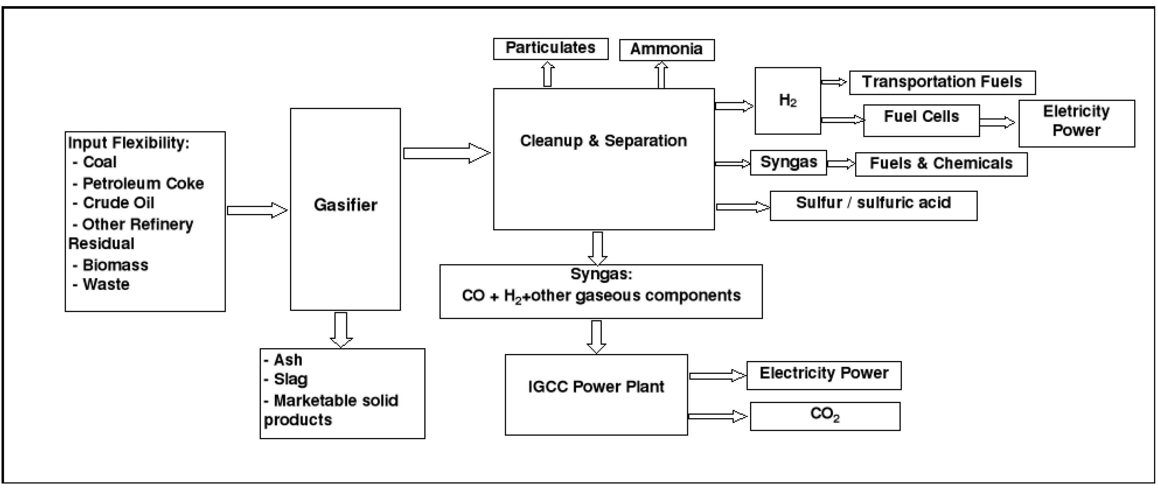
Similarly, gasification is the starting point for getting transportation fuels. There are basically two methods:

• The Fischer-Tropsch (FT) liquefaction technology was developed in 1920 by Franz Fischer and Hans Tropsch. It was later used during the II World War by Germany and Japan. More lately, it has been intensely used in South Africa, where it provides some 28% of the diesel and gasoline needs. The FT process is also used for converting syngas to other products such as naphtha, waxes, ammonia, hydrogen and methane. The syngas is reacted in the presence of an iron or cobalt catalyst7.
• Another process is the so-called Methanol to Gasoline (MTG). The syngas is first transformed into methanol and this in turn into gasoline. This technology was developed for use by ExxonMobil in New Zealand during the 1980s and can produce commercial levels of transportation fuels.

Figure 1 shows entry and exit flexibility for both gasification and liquefaction processes. This flexibility has important economic consequences which are explored in this paper.

3. Coal Reserves and World Consumption: The Security of Supply

Coal reserves represent about 70% of the world’s proven fossil resources, and they are geographically more delocalized than gas or oil (see Table 2)8. Its usage can improve the security of energy supply, for example when it comes to the reduction in natural gas imports. The extended utilisation of coal could also alleviate the pressure on the demand for other alternative fuels like natural gas. To make this possible, though, the gasification technology needs to be further developed and optimized.

Figure 1. Input and output flexibility in gasification technology.

Figure 1. Input and output flexibility in gasification technology.

The ratio of proven reserves to production (R/P) at the end of 2008 appears in Table 3 for different geographic areas (BP [9]). We also include the R/P ratio for natural gas since we will refer to this fuel in Section 4.

As can be seen in Figure 2, coal consumption has increased substantially at the world level. Countries such as China satisfy a significant part of their energy needs with coal. Right now efficiency enhancement ranks higher than before. This is for the sake of lower coal consumption and specific emission, as well as better economics.

With regard to future consumption, according to the Reference Scenario in IEA [10] coal sees the biggest increase in demand in absolute terms, jumping by 73% between 2005 and 2030 and pushing its share of total energy demand up from 25% to 28%. Similarly, in the EIA [11] reference case, world coal consumption increases by 49% from 2006 to 2030, and coal’s share of world energy consumption increases from 27% in 2006 to 28% in 2030.

4. Relevant Issues for an Economic Assessment

From an economic viewpoint, the following issues are relevant when assessing gasification: (a) the price of the input fuels9; (b) the efficiency of the generation processes; (c) the flexibility regarding alternative fuels; (d) the flexibility concerning output products; (e) the availability and reliability of the system; (f) the environmental costs related to gasification technologies; (g) the option to install a CCS facility alongside the gasification plant; (h) the total capital cost; (i) construction time10; (j) annual maintenance costs; (k) the project lifetime; (l) other additional items (water consumption, disposal of pollutants such as mercury, etc.). These aspects are elaborated below.

4.1. Fuel cost without entry flexibility in an IGCC plant

Before addressing the valuation of input flexibility, first we consider the case in which only one fuel can be used as feed material in the IGCC power plant. It could be coal or any other fuel input; for example, refineries produce amounts of crude oil residual. This low-cost fuel might be used in the IGCC plant to produce only power or both power and hydrogen (in this case there would be output flexibility).

Table 2. Recoverable coal resources around the world (million short tons). Source: see note 8.

Country	Anthracite and	Lignite and	Total
	Bituminous	Subbituminous	Recoverable Coal
Canada	3,826	3,425	7,251
United States	122,001	141,780	263,781
Others North America	948	589	1,537
North America	126,776	145,793	272,569
Brazil	0	7,791	7,791
Colombia	7,251	420	7,671
Others Central & South America	718	1,761	2,479
Central & South America	7,969	9,973	17,941
Former Serbia and Montenegro	7	15,299	15,306
Germany	168	7,227	7,394
Poland	6,627	1,642	8,270
Others Europe	2,495	17,317	19,812
Europe	9,296	41,485	50,781
Kazakhstan	31,052	3,450	34,502
Russia	54,110	118,964	173,074
Ukraine	16,922	20,417	37,339
Others Eurasia	1,102	3,100	4,202
Eurasia	103,186	145,931	249,117
Middle East (Iran)	1,528	0	1,528
South Africa	52,911	0	52,911
Others Africa	1,577	192	1,769
Africa	54,488	192	54,680
Australia	40,896	43,541	84,437
China	68,564	57,651	126,215
India	57,585	4,694	62,278
Others Asia & Oceania	2,950	7,927	10,877
Asia & Oceania	169,994	113,813	283,807
World Total	473,236	457,186	930,423

Table 2. Recoverable coal resources around the world (million short tons). Source: see note 8.

Country	Anthracite and	Lignite and	Total
	Bituminous	Subbituminous	Recoverable Coal
Canada	3,826	3,425	7,251
United States	122,001	141,780	263,781
Others North America	948	589	1,537
North America	126,776	145,793	272,569
Brazil	0	7,791	7,791
Colombia	7,251	420	7,671
Others Central & South America	718	1,761	2,479
Central & South America	7,969	9,973	17,941
Former Serbia and Montenegro	7	15,299	15,306
Germany	168	7,227	7,394
Poland	6,627	1,642	8,270
Others Europe	2,495	17,317	19,812
Europe	9,296	41,485	50,781
Kazakhstan	31,052	3,450	34,502
Russia	54,110	118,964	173,074
Ukraine	16,922	20,417	37,339
Others Eurasia	1,102	3,100	4,202
Eurasia	103,186	145,931	249,117
Middle East (Iran)	1,528	0	1,528
South Africa	52,911	0	52,911
Others Africa	1,577	192	1,769
Africa	54,488	192	54,680
Australia	40,896	43,541	84,437
China	68,564	57,651	126,215
India	57,585	4,694	62,278
Others Asia & Oceania	2,950	7,927	10,877
Asia & Oceania	169,994	113,813	283,807
World Total	473,236	457,186	930,423

Even when the IGCC plant is designed to run on a single fuel, it would be possible to choose fuels that are less suited for plants that burn pulverized coal (PC). For instance, PC plants—to comply with environmental regulations—would be required to use coal with a low sulfur content, or to adopt post combustion removal systems (such as flue gas desulphurizer or spray dry scrubber). On the other hand, IGCC technology allows for a cheaper capture of carbon (or sulfur). In connection with this technology, the type of fuel burnt can affect both capital costs and operation costs of the plant.

Table 3. Proven reserves to production ratio ($R/P$) at end of 2008.

Area	Coal	Area	N.Gas
Total North America	216	Total North America	10.9
Total S. & Cent. America	172	Total S. & Cent. America	46.0
Total Europe & Eurasia	218	Total Europe & Eurasia	57.8
Total Middle East & Africa	131	Total Middle East	>100
Total Asia Pacific	64	Total Africa	68.2
TOTAL WORLD	122	Total Asia Pacific	37.4
of which: European Union	51	TOTAL WORLD	60.4
OECD	164	of which: European Union	15.1
Former Soviet Union	433	OECD	14.6
Other Emerging Mkt. Econ.	60	Former Soviet Union	71.8

Source: BP Statistical Review of World Energy 2009.

Table 3. Proven reserves to production ratio ($R/P$) at end of 2008.

Area	Coal	Area	N.Gas
Total North America	216	Total North America	10.9
Total S. & Cent. America	172	Total S. & Cent. America	46.0
Total Europe & Eurasia	218	Total Europe & Eurasia	57.8
Total Middle East & Africa	131	Total Middle East	>100
Total Asia Pacific	64	Total Africa	68.2
TOTAL WORLD	122	Total Asia Pacific	37.4
of which: European Union	51	TOTAL WORLD	60.4
OECD	164	of which: European Union	15.1
Former Soviet Union	433	OECD	14.6
Other Emerging Mkt. Econ.	60	Former Soviet Union	71.8

Source: BP Statistical Review of World Energy 2009.

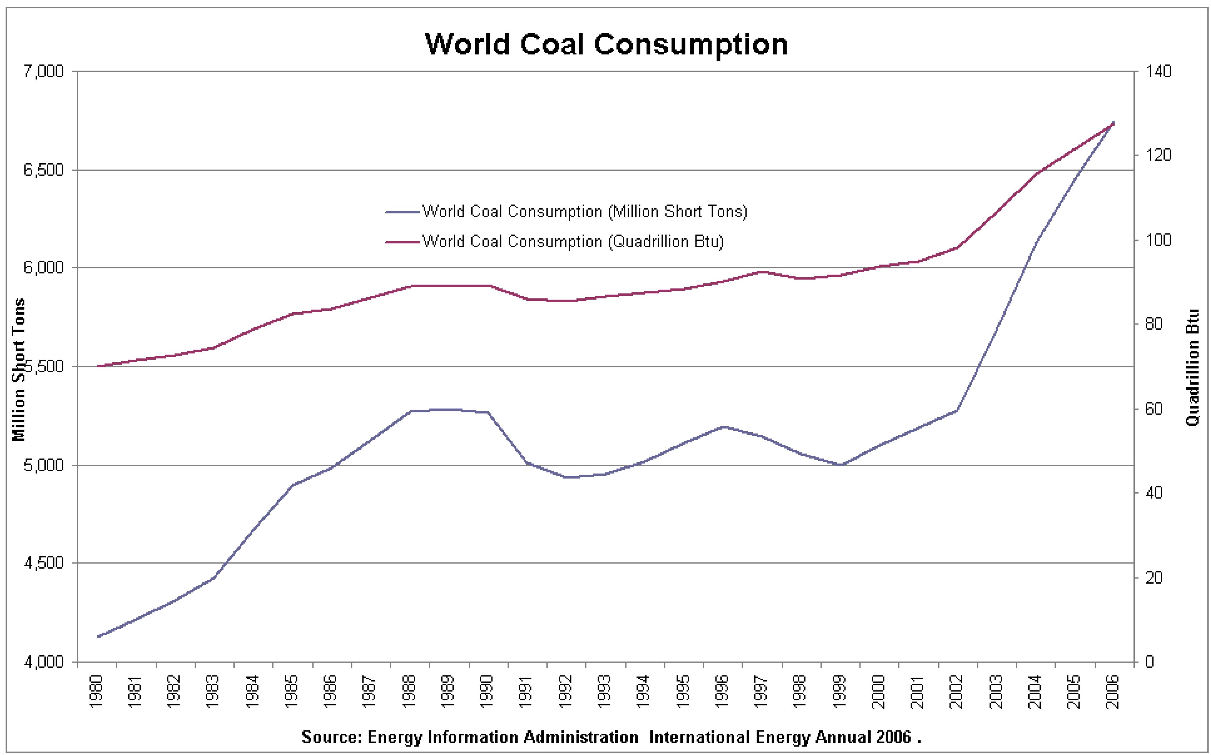
Figure 2. World consumption of coal. Source: EIA.

Figure 2. World consumption of coal. Source: EIA.

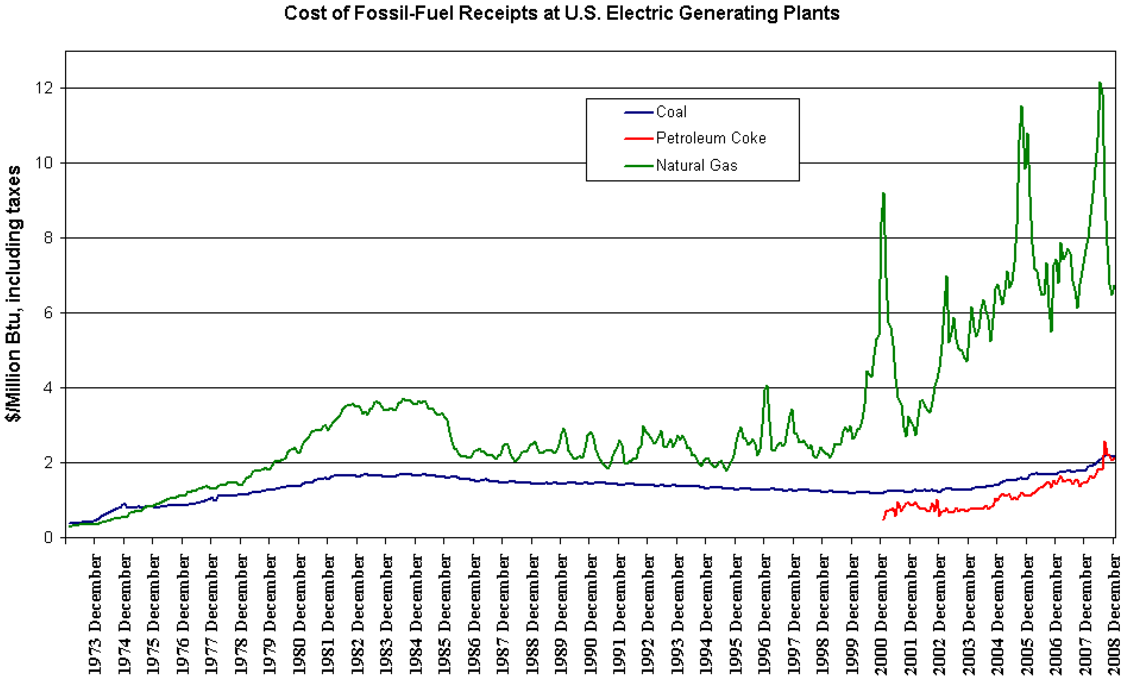
The price of the fuel used to produce one megawatt-hour (MWh) of electricity is one of the main advantages of the IGCC technology over other competing alternatives. Figure 3 shows the costs of U.S. power plants in nominal U.S. dollars. Coal and petroleum coke (or petcoke) enjoy a significant advantage over natural gas for a given power generation efficiency. This comparative advantage has increased steeply over the last years11.

Figure 3. Cost of several fossil fuel inputs to electricity production in the U.S. Source: U.S. DoE.

Figure 3. Cost of several fossil fuel inputs to electricity production in the U.S. Source: U.S. DoE.

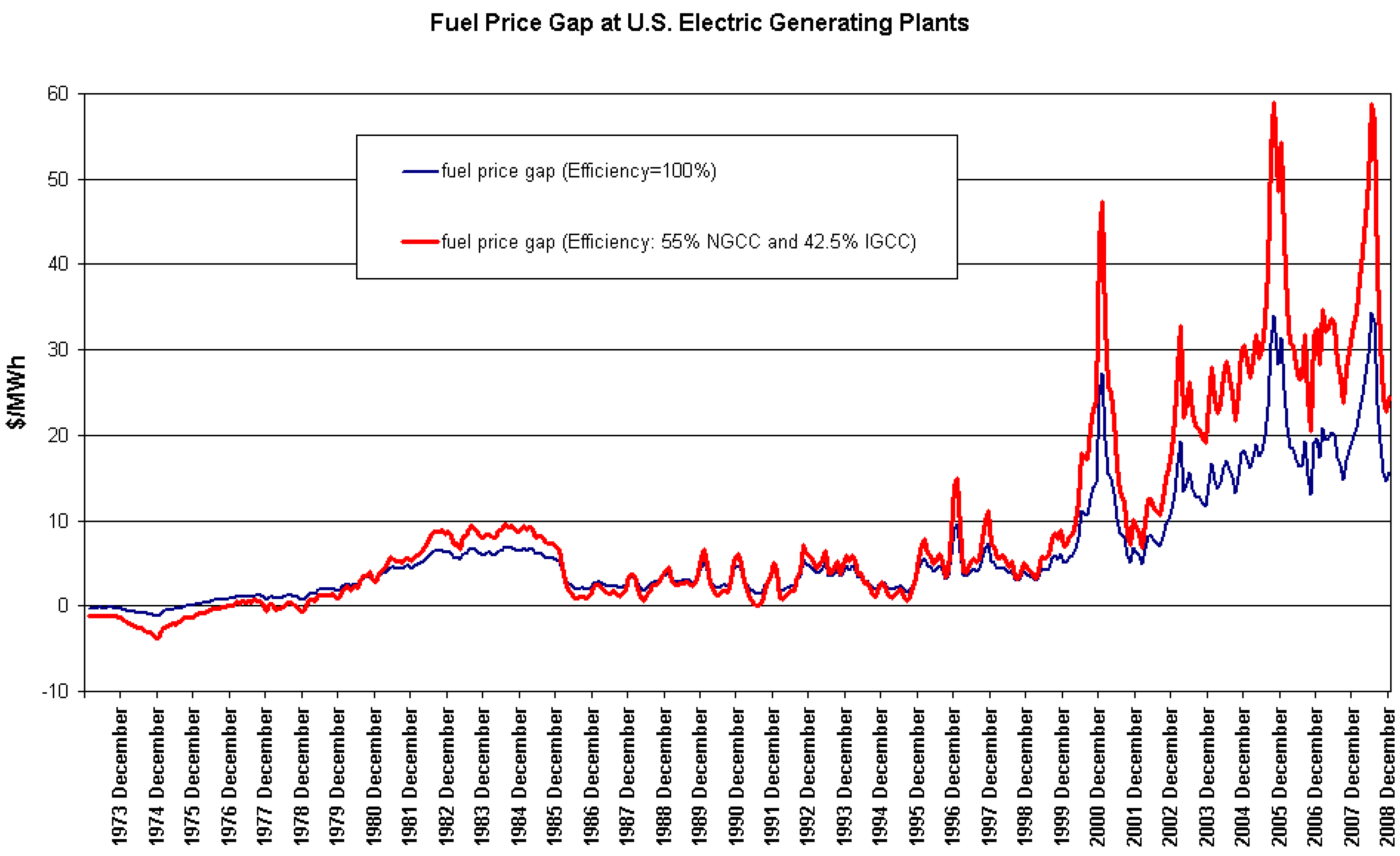
Figure 4 shows the fuel price gap (again in nominal U.S. dollars) between coal and natural gas for producing one MWh with standard efficiency levels at both IGCC and NGCC power plants, 42.5% and 55% respectively. It can be seen that high gas prices impact strongly this technology’s variable costs, a fact which is not offset by its higher efficiency level.

The greater fuel flexibility afforded by gasification technologies can be an important source of value: at any time it allows choosing the cheapest alternative (within the limits established by the specific design of each gasification plant). The IGCC technology must incur lower variable costs linked to fuel consumption than the NGCC technology; in particular, the fuel costs of producing one unit of electricity must be lower. At the same time, by using a gas turbine and a steam turbine, the IGCC plant reaches higher efficiencies than a conventional coal-fired plant. Thus we have:

$$\frac{P_G}{E_G}>\frac{P_C}{E_C}>\frac{P_C}{E_{IGCC}},$$

where $P_G$ and $P_C$ denote the price of natural gas and coal, respectively. $E_G$ and $E_C$ stand for the thermal efficiency of a NGCC plant and a PC plant, while $E_{IGCC}$ applies to the IGCC plant. For the sake of simplicity, we assume that all the prices have been converted into $/MWh (or €/MWh).

Therefore, the difference $\frac{P_G}{E_G}-\frac{P_C}{E_{IGCC}}$ measures the relative (cost) advantage of an IGCC plant over an NGCC plant in terms of the fuel used. Its advantage over a PC plant is attributed to its higher efficiency: $P_C(\frac{1}{E_C}-\frac{1}{E_{IGCC}})$12. The advantage provided by the fuel price gap (adjusted for relative efficiencies) must be assessed numerically as an input to decision making process. Especially, it is important to know if this advantage, when added to any other that could be exploited, allows to compensate for some disadvantages, such as the higher investment costs. Specific items to be considered include fuel prices, installations’ efficiencies, and their expected useful lives.

Figure 4. Fuel price gap between natural gas and coal.

Figure 4. Fuel price gap between natural gas and coal.

Obviously, since we are dealing with long-lived facilities, their value depends not only on current prices and price gaps for producing one MWh, but on their future levels as well. Present and future coal reserves, refinery production processes, the evolution of demand and extraction costs, they all affect the future price gap, which can turn out to be very different from that prevailing in the spot market currently. Futures markets can be particularly helpful in this respect.

Figure 5 shows the prices of futures contracts on natural gas and coal on the New York Mercantile Exchange (NYMEX). As could be expected, natural gas prices display a prominent seasonal pattern on any given day. However, in a long-term evaluation, when gas is consumed on a uniform basis to produce electricity, using the deseasonalised series (also shown) would be enough. Currently traded contracts’ maturities go beyond 2020. Note also that these prices depend on local conditions and can be the object of speculation to some degree.

Futures prices are not the spot prices expected to prevail in the physical or actual world in the future, which are harder to estimate (because of the risk premium embedded in actual prices). A standard result in Finance textbooks is that the futures price for a given maturity is equal to the spot price expected to prevail at that time if market agents are assumed to be risk neutral. Thus, the futures price provides the expected value of the future spot price in a risk-neutral world; and it can be properly discounted to the present at the risk-free interest rate. Figure 6 shows the futures price gap for the same efficiency levels as before (namely 42.5% and 55%). Therefore, the gap in this figure corresponds to the gap in a risk-neutral world. The fuel price gap is given by:

$$\frac{P_G}{E_G}-\frac{P_C}{E_C}=\frac{P_G}{0.55}-\frac{P_C}{0.425}.$$

Figure 5. Price of futures contracts on natural gas and coal. Source: NYMEX.

Figure 5. Price of futures contracts on natural gas and coal. Source: NYMEX.

The information embedded in the prices of futures contracts on coal and natural gas can be used to assess the present value of energy costs. Thus, by using readily available futures prices and discounting them at the riskless rate, we can derive the present value of cumulative costs (or revenues) in a relatively simple manner, even graphically. Stated differently, we do not need to compute the actual price process nor to discount future values at a rate augmented by the risk premium.

In particular, we can fit a curve to the discrete futures prices available in the market for a set of maturities (say March, June, September, December, up to five years ahead)13. Let $F(t,0)$ denote this curve, which shows the time-0 price of a unit of energy (conveyed in coal, or gas) to be delivered at time t in exchange for an amount of money $F(t,0)$. The curve $F(t,0)$ on a given date (0) can be fitted by following several procedures14. This will allow us to compute the value V at that time (0) of future fuel costs15:

$$V_{{\tau }_1,{\tau }_2}=\frac{1}{E}{\int }_{{\tau }_1}^{{\tau }_2}{e}^{-rt}F(t,0)dt.$$

(8)

E denotes the thermal efficiency of the plant involved; it inversely affects the input consumption per unit of output. Depending on the particular type of plant (natural gas-fired, or coal-fired, or IGCC), E can take on the value $E=\left\{E_G,E_C,E_{IGCC}\right\}$. We are accordingly interested in the futures price of either natural gas or coal, i.e., $F(t,0)=\left\{F_G(t,0),F_C(t,0)\right\}$. The time limits of the integral, ${\tau }_1$ and ${\tau }_2$, comprise the useful life of the plant16. The integral stands for the (time-0) present value of the costs incurred by producing a unit of energy (e.g., one MWh/year) from natural gas or coal over the plant lifetime ${\tau }_2-{\tau }_1$. Each futures price (of natural gas, or coal) paid at time t is discounted at the risk-free interest rate r over the time period stretching from now (time 0) until the contract’s maturity date (t)17. Several cases can be analysed within this framework.

Figure 6. Fuel price gap as implied by futures prices of natural gas and coal.

Figure 6. Fuel price gap as implied by futures prices of natural gas and coal.

Case 1. Assume that a given design mix of fuel inputs is used every year in an IGCC plant. For example, each unit of black coal is accompanied by a fixed number α of units of petroleum coke. Our formula for the present value of future fuel costs would then become:

$$V_{{\tau }_1,{\tau }_2}=\frac{1}{E_{IGCC}}\left[{\int }_{{\tau }_1}^{{\tau }_2}{e}^{-rt}{F}_C(t,0)dt+\alpha {\int }_{{\tau }_1}^{{\tau }_2}{e}^{-rt}{F}_{PC}(t,0)dt\right],$$

where $F_{PC}(t,0)$ stands for the futures price of petroleum coke to be delivered at t.

Case 2. In principle the above formula is also valid for computing the present value of a unit of electricity (one MWh) to be produced each period over the plant life ${\tau }_2-{\tau }_1$. If there were a well-developed futures market for electricity then we could take the futures price $F_E(t,0)$ on this market. The present value of future revenues from electricity would be:

$$V_{{\tau }_1,{\tau }_2}^E={\int }_{{\tau }_1}^{{\tau }_2}{e}^{-rt}{F}_E(t,0)dt.$$

Case 3. Let us consider two different power plants designed to produce the same yearly amount of electricity18. They are further assumed to have the same useful life, and to start operation at the same time. In this case, the above present value of revenues would not be a relevant input to the investment decision provided it is high enough to recover the investment costs and enjoy a reasonable profit. Instead, the relevant factor would be cost minimization across plants while taking into account investment risks.

4.2. Fuel flexibility in an IGCC power plant

In fact, not one but a wide variety of feedstocks is available to an IGCC station: coal, biomass, petroleum coke, crude oil, high sulfur fuel oil, other refinery residuals. Some of these feedstocks are not suitable for the use in combustion power generation cycles considering the potential pollution risks. This input flexibility is an intrinsic feature of IGCC plants as compared to other power generation technologies. For example, a flexible design for a PC plant to run on several types of coal would command a much higher price and entail a greater complexity of the plant.

We have just seen above the case without input flexibility. There were more than one input fuel on offer, but we were restricted to choose only one fuel type to be used as a feedstock from the opening of the plant to its closure. We have shown that in this case futures markets alone can allow us to compute the present values of alternative fuel costs. However, under input flexibility the true cost to be incurred will be somewhat lower, given that at some times we will be able to select another, cheaper fuel. In other words, the option to switch between fuels adds an economic value to the power station, since at every moment the cheapest alternative can be chosen. Note, though, that all the ensuing effects of any fuel switching must be duly taken into account. For instance, there may be a switching cost to fuel substitution, or the plant efficiency level may fall short of the design level. Nonetheless, it is an important option since, for installations with long life spans, the cost of the potential fuels may undergo significant changes over time.

Thus, let us consider a hypothetical scenario in which the plant managers can choose between using coal or petcoke19. The thermal efficiency changes accordingly ($E_{IGCC}^C$ or $E_{IGCC}^{PC}$). There are switching costs between fuels20: $I(c\to pc)$ denotes the costs to switching from coal to petcoke, whereas $I(pc\to c)$ is the cost to switching from petcoke to coal.

First let us focus on the revenue side. The power plant is designed to produce an annual electricity output A (in MWh). This value is a function of the installed capacity, M (in MW), and the fraction of the year that the plant is expected to be in operation, defined as capacity factor, C (with $0\le C\le 1$):

$$A=M\times 365\times 24\times C=8760MC.$$

If the capacity factor C changes over time, as it actually does, then we should use a sum over the whole year:

$$A=\sum _{t=0}^{8760}MC\left(t\right)\Delta t.$$

This electricity is assumed to be sold every year on the futures market at the current (exogenous) market price (in €/MWh). Once we have derived the yearly revenues, we can compute their cumulative value.

Next we focus on fuel costs. If the prices of both fuels are $P_C$ and $P_{PC}$ (in €/MWh), then total fuel costs over a period $\Delta t$ would amount to $F{C}_C=A\Delta t{P}_C/E_{IGCC}^C$ if the plant is operated in coal mode, and $F{C}_{PC}=A\Delta t{P}_{PC}/E_{IGCC}^{PC}$ if it is operated in petcoke mode. Now we address the minimization of the costs of running the plant over the whole time horizon by means of two bi-dimensional binomial lattices, one for each mode of operation. To understand what a (one-dimensional) binomial lattice is, we can think of a random variable (say, a price P) that begins at a known value ($P_0$), and may increase (by a multiplicative factor u) with a given probability to $uP$ or decrease with complementary probability to $dP$ (where $d=1/u$) at the end of the period $\Delta t$. This same process follows over successive periods. The term ’bi-dimensional’ just indicates that we are not dealing with one but two random prices at any moment. Thus, we have a given combination of prices ($P_C$ and $P_{PC}$) at the initial node. Each of the prices evolves on its own so there are four branches starting from the initial node. At the end of the period there are four possible nodes: (1) both prices have moved up, (2) the first one up and the second down, (3) the first one down and the second up, or (4) both prices have moved down.

Prior to the valuation of future costs we must know how fuel prices behave in a risk-neutral world (for example, by exploiting futures prices), along with their volatilities and correlations (these estimates must be consistent with futures market data). This all will allow us to compute the changes $\Delta X_C$ and $\Delta X_{PC}$ in the log prices of both fuels (i.e., $X_C\equiv ln{P}_C$ and $X_{PC}\equiv ln{P}_{PC}$) and the risk-neutral probabilities $p_{uu}$, $p_{ud}$, $p_{du}$, $p_{dd}$; for one, $p_{ud}$ is the probability (in the risk-neutral world) that after a short time lapse, $\Delta t$, coal price has moved upwards while petcoke price has moved downwards.

The way to proceed in our case is by using not one but two binomial lattices, one for each of the two possible modes of operation. At any moment the manager of the plant must compare the value in a given node of one lattice (mode) with its counterpart in the other lattice (mode) after adjusting for any switching cost. In this way she can choose the optimal mode of operation at any time. Valuation proceeds backwards, from the end of the useful plant life to the moment when the investment decision is made (see Abadie and Chamorro [6]).

At expiration the IGCC plant ceases fuel consumption, so it incurs no fuel costs ($W=0$), irrespective of whether it expires operating in coal mode or petcoke mode21. Therefore, when the plant reaches maturity:

$$W_C=0;W_{PC}=0.$$

In other words, the fuel costs at the final nodes in both the coal-mode lattice and the petcoke-mode lattice are zero.

In earlier periods production costs must be minimized by choosing between two alternatives:

• to continue operation in the current mode during the period $\Delta t$:

  -

  paying for the fuel costs,

  -

  and accept the present value of the future costs that derive from starting the next period in the current mode, assuming that at any time in the future the best mode of operation will be chosen;

• to change the operation mode:

  -

  incurring the switching costs,

  -

  operate in the new mode during $\Delta t$, paying for the fuel costs,

  -

  and accept the present value of the future costs that derive from starting the next period in the current mode, assuming that at any time in the future the best mode of operation will be chosen.

Analytically, when the starting state corresponds to operating with coal, the binomial lattice will take on the following value:

$$\begin{array}{cc}\hfill W_C& =min[F{C}_C+e^{-r\Delta t}(p_{uu}{W}_C^{uu}+p_{ud}{W}_C^{ud}+p_{du}{W}_C^{du}+p_{dd}{W}_C^{dd}),\end{array}$$

$$\begin{array}{cc}& I(c\to pc)+F{C}_{PC}+e^{-r\Delta t}(p_{uu}{W}_{PC}^{uu}+p_{ud}{W}_{PC}^{ud}+p_{du}{W}_{PC}^{du}+p_{dd}{W}_{PC}^{dd})].\end{array}$$

(9)

In words, starting in coal mode (hence $W_C$), fuel cost over the period $\Delta t$ will be the minimum of two quantities: (1) the cost to continue operation in the current (coal) mode during that period, paying for the fuel costs ($F{C}_C$), and accepting the present value of the future costs that derive from starting the next period in the current mode (i.e., the expected value of the four possible nodes discounted at a rate r over that period), and (2) the cost to change the operation mode (to petcoke), incurring the switching costs ($I(c\to pc)$), operate in the new mode during that period, paying for the fuel costs ($F{C}_{PC}$), and accept the present value of the future costs that derive from starting the next period in the current mode (the last term with the discount factor).

Similarly, when the starting state corresponds to operating in petcoke mode, the binomial lattice will take on the following value:

$$\begin{array}{cc}\hfill W_{PC}& =min[F{C}_{PC}+e^{-r\Delta t}(p_{uu}{W}_{PC}^{uu}+p_{ud}{W}_{PC}^{ud}+p_{du}{W}_{PC}^{du}+p_{dd}{W}_{PC}^{dd}),\end{array}$$

$$\begin{array}{cc}& I(pc\to c)+F{C}_C+e^{-r\Delta t}(p_{uu}{W}_C^{uu}+p_{ud}{W}_C^{ud}+p_{du}{W}_C^{du}+p_{dd}{W}_C^{dd})].\end{array}$$

(10)

Following this process backwards we arrive at the initial moment (time 0). Then we choose the cheapest alternative:

$$min(W_C,W_{PC}).$$

Thus we learn how to start operation of the plant, whether running on coal or petcoke. Besides, as fuel prices evolve over time, we can trace their movements on the two lattices. They already show when and where it is optimal to switch fuel, so we can react accordingly. In this way we minimize the fuel cost of running the plant over time.

Whether the “initial” least-cost fuel (as opposed to the alternative of using one single fuel forever) is coal or petcoke depends on several factors: (i) switching costs: the higher they are, the less valuable the option to switch; (ii) fuel prices volatilities: if there is no uncertainty, we are in a deterministic setting so the option to switch becomes worthless; (iii) fuel prices correlation: if they are highly unrelated, there is a greater chance that the option to switch to the cheaper fuel will be exercised at same time in the future; (iv) the (efficiency-adjusted) gap between both fuel prices: the lower it is, the higher the probability that price swings will entail changes in their relative cost and economic appeal.

4.3. Availability and reliability of the IGCC plant

Given that the IGCC plant commands a higher investment cost, the percentage of time over which the plant operates is particularly relevant from an economic point of view. According to Chen and Rubin [12], the assumed capacity factor contributes most to the total volatility of the cost of electricity in their analysis. An operating plant produces electricity and hence revenues that can meet both fixed and variable costs and also service the debt. Typically, funding needs will require the payment of an interest rate which is above the risk-free rate r.

Due to its characteristics, it would be sensible to design the IGCC plant as a base load plant. Thus, a 400 MW plant which operates 70% on average over the year would produce 2,452,800 MWh yearly. If, instead, the availability rises to 80%, then the production would rise to 2,803,200 MWh yearly. This is 350,400 MWh more over a year. A gross computation suffices to show the importance of the improvement. We just multiply this amount by the profit spread (per MWh) and the number of years of useful life. After discounting the resulting figure to the present, we would see that this present value is sizeable.

The higher complexity of the IGCC plant (relative to other power generation alternatives) involves a risk that the desired availability is not reached. This is why the time in operation is one of the features to look after carefully, so as to improve the plant’s profitability. Indeed, notwithstanding some successful experiments in IGCC power plants, the low number of operating plants showed a lot of problems, mostly concerning the availability (Franco and Diaz [8]). Indeed there are several reasons for concern. One is fluctuations of demand over time. At a higher level, there is a need to keep thermal plants running at some degree for various reasons (e.g., to provide greater reliability and stability of the whole system). Therefore, not all units in that system can be operated at full output. In sum, really high availabilities may not be possible in practice.

The importance of availability goes well beyond the amount of output electricity. It affects more fundamental parameters, among them the efficiency of the plant. Net design energy efficiency (also called name-plate efficiency) is a static energy efficiency and gives the energy efficiency if a plant operates at best performance. The operational energy efficiency is the year-round average efficiency of a plant and is usually a few percent points lower than the design efficiency. Capacity utilization is an important factor influencing the operational efficiency of a plant. According to Graus and Worrell [13], operational efficiency is typically 1–2% lower than the design energy efficiency if the plant operates at 85% capacity (7500 full load hours). If the power plant operates at 50% capacity the operational efficiency is typically 3–4% lower. Efficiency, in turn, affects fuel consumption (for a given output) and pollutant emissions.

4.4. Environmental costs of gasification technology

Here we restrict ourselves to ${\mathrm{CO}}_2$ emissions and their economic cost as perceived through the market for carbon emission allowances; other pollutants are considered in Section 5. Even though an IGCC plant may have been granted a number of free allowances initially, the very existence of this market implies that at some point in time selling (some or all of) them can be the best decision. Note, however, that the possibility of auctioning (as opposed to “grand-fathering”) the allowances beyond Kyoto (2013–2020) looks ever more likely. Under these circumstances, unless a temporary support to this technology is in place (e.g., because of its innovative profile), the cost of emission allowances should be taken into account.

Actual emissions will depend mainly on the plant efficiency. The first plants deployed reach efficiencies between 39% and 43%. Under current technology, however, efficiency can presumably reach 50%, with even 60% being possible in the future. For example, according to IPCC [14] a plant burning bituminous coal has an emission factor of 94.6 k${\mathrm{CO}}_2/GJ$ under 100% efficiency conditions. Thus total emissions amount to 0.34056 t${\mathrm{CO}}_2/MWh$ under full efficiency22. Therefore, emissions could change as a function of efficiency as shown in Table 4.

Table 4. Carbon emissions (t${\mathrm{CO}}_2/MWh)$ as a function of efficiency (%).

	35%	40%	45%	50%	55%	60%
Emissions from IGCC	0.973	0.851	0.757	0.681	0.619	0.568
Emissions from NGCC	-	-	-	0.404	0.367	0.337
Difference	-	-	-	+0.277	+0.252	+0.231

Table 4. Carbon emissions (t${\mathrm{CO}}_2/MWh)$ as a function of efficiency (%).

	35%	40%	45%	50%	55%	60%
Emissions from IGCC	0.973	0.851	0.757	0.681	0.619	0.568
Emissions from NGCC	-	-	-	0.404	0.367	0.337
Difference	-	-	-	+0.277	+0.252	+0.231

Higher efficiencies not only translate into fuel savings (and hence a weaker market demand for fuel), but lower emissions and spared allowances as well (i.e., lower environmental costs). Carbon emissions are certainly a relatively heavier burden for IGCC than for gas-fired combined cycles. Yet the difference narrows for higher efficiency levels23.

As long as NGCC plants continue to set the market price of electricity ever more frequently, they will eventually pass their costs on to this price. Since natural gas is more expensive than the fuels used in an IGCC plant, this is an advantage of the latter. And conversely, the IGCC plant may find it difficult to pass their carbon costs on to the electricity price; this is a comparative disadvantage. This handicap to the gasification technology can be lessened in two ways: a higher level of efficiency and, beyond some threshold level of carbon price, the construction of a carbon capture and storage (CCS) unit24.

Now the European Union Emissions-Trading Scheme (EU ETS) is a market for carbon permits. It commenced operation in 2005. The sectors covered by the system are power generation and energy-intensive manufacturing industry (from 2011/2012, also aviation). The cap on emission allowances will be cut by 21% in 2020 in comparison to 2005 levels (European Commission [15]).

Let $F_{EMI}(t,0)$ be the time-0 curve in the market for futures contracts on emission allowances. Usually this curve shows an increasing profile over time (within a given trading period, e.g., the Kyoto commitment period 2008–2012). This is mainly due to a growing demand and a constant supply of permits. Future cuts in the total cap of allowances will probably entail a jump in prices. The futures curve would ideally reflect all these issues and it would fit neatly the market prices in place on the day we undertake the valuation.

Since every t${\mathrm{CO}}_2$ emitted bust be met by one emission allowance, the present value of emitting one t${\mathrm{CO}}_2$ yearly over the plant’s useful life is:

$$V_{{\tau }_1,{\tau }_2}^{EMI}={\int }_{{\tau }_1}^{{\tau }_2}{e}^{-rt}{F}_{EMI}(t,0)dt.$$

This cost must be multiplied by the total number of tonnes emitted yearly. For example, if the plant size is 400 MW and it operates 80% of the time (admittedly, a tall order), it will produce 2,803,200 MWh/year. Now, if it burns bituminous coal with an efficiency of 45% it will emit 0.757 t${\mathrm{CO}}_2/MWh$, or 2,122,022 t${\mathrm{CO}}_2/$year; this figure must multiplied by the above cost. Depending on the emission allowance price, the impact on the plant’s profitability can be significant. 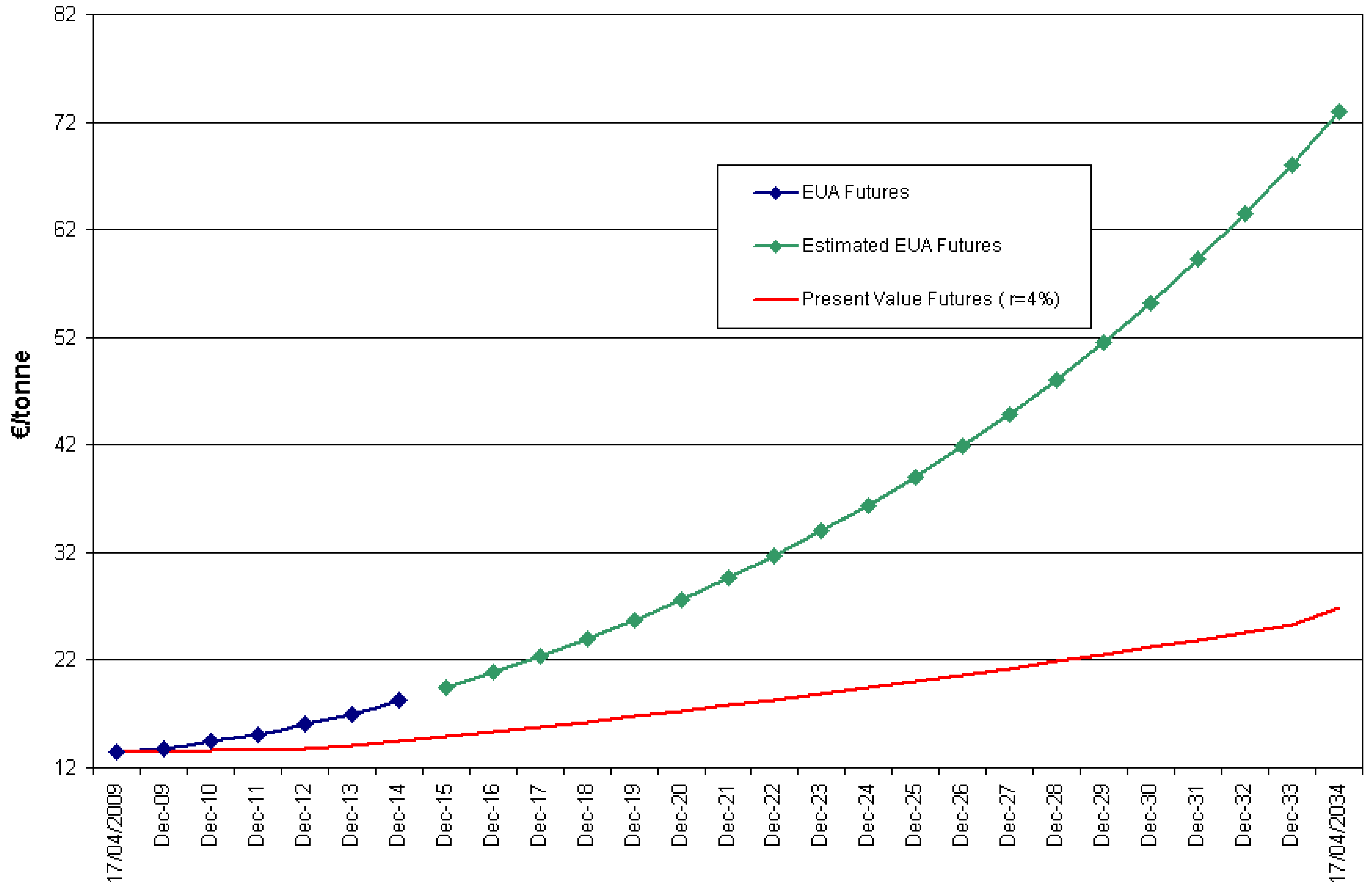Figure 7 shows futures prices on the European Climate Exchange (ECX) on 04/17/200925. Futures contracts currently traded have maturities stretching until December 2014. Beyond this date, some extrapolation method must be used.

Figure 7. Futures prices of European Union emission allowances (blue line), estimated prices for the distant future (green line), and futures prices discounted to the present (red line). Source of EUA prices: ECX.

Figure 7. Futures prices of European Union emission allowances (blue line), estimated prices for the distant future (green line), and futures prices discounted to the present (red line). Source of EUA prices: ECX.

On the other hand, increasing efficiency up to 50%, would take emissions down to 0.681 t${\mathrm{CO}}_2$/MWh, or 1,908,979 t${\mathrm{CO}}_2/$year. In this case 213,043 t${\mathrm{CO}}_2/$year have been avoided. This figure is not to be overlooked, since it amounts to savings of 10% in the bill of carbon permits, plus the simultaneous savings in fuel consumed.

A previous experience of emissions markets can be found in the U.S. Clean Air Act (the Acid Rain Program). Insley [16] addresses the effect of uncertainty in the price of emission permits on the decision to install a “scrubber”. To model this uncertainty, she proposes a geometric Brownian motion (GBM) for the changes in the permit price. At the same time, observation of Figure 7 suggests that, for the contracts available, futures prices of carbon allowances grow exponentially with the time to maturity; this is consistent with a GBM process. Therefore, if we want a simple estimation of carbon costs, we can assume that the allowance price follows a standard GBM; see Section 6 below for details. Then, the formula for the futures price reduces to:

$$F_{EMI}(t,0)=C_0{e}^{{\alpha }^{*}t},$$

(11)

where $C_0$ denotes the allowance price at time 0 (when the valuation is made), and ${\alpha }^{*}$ is the drift rate of the allowance price process. It can easily be shown that beyond 2014 (the latest maturity now traded), assuming that the same GBM process as over 2008-2012 applies, the futures price is given by:

$$F{(t,0)}_{EMI}=F{(14,0)}_{EMI}\times e^{{\alpha }^{*}(t-14)},t\ge 14.$$

Computing the drift rate through the difference of the (log) prices for maturities December-2013 and December-2014, ${\alpha }^{*}=lnF(14,0)-lnF(13,0)$, the lower curve in Figure 7 results. This curve depicts $e^{-rt}{F}_{EMI}(t,0)$ for a (nominal) riskless interest rate $r=4$% assumed in the long term. Therefore, the area below this curve over the next 25 years is:

$$V_{0,25}^{EMI}={\int }_0^{25}{e}^{-rt}{F}_{EMI}(t,0)dt.$$

The amount $V_{0,25}^{EMI}$ gives the present value of the cumulative cost of emitting one metric t${\mathrm{CO}}_2$ each year over the next quarter century. The present value of total carbon costs equals $V_{0,25}^{EMI}$ times the total number of tonnes emitted yearly26.

4.5. Facilities’ cost

Estimating installation costs is not an easy task. In particular, it depends on the specific country in which the IGCC plant is built, because of the different costs of labor, capital, materials, taxes, potential subsidies or support measures, etc. Total cost is particularly sensitive to the evolution of the prices of the commodities used during construction (steel, cement, ...); these prices have been rising sharply until recently thus pushing costs to new heights. Note also that there could be economies of scale when building bigger gasification plants. These economies, though, must be weighed against the value of modularity.

There are distinct estimates of facility costs. In general they are not consistent with each other, given that they rest on very different assumptions. Yet it is worth noting that, in the medium term, the U.S. Department of Energy (DoE) sets a target capital cost of less than $1,000/kW for IGCC plants. Irrespective of the higher cost of the first IGCC stations, Table 5 shows some estimates for the mid term and compares them with those of alternative Super Critical PC plants and Ultra Super Critical PC plants.

Table 5. Capital cost ($/kW) for different plants.

	IGCC	SCPC	USCPC
DoE	1,300	1,000-1,400	-
Harvard	1,400	1,200	-
EPRI	1,350	-	1,235
Flour	1,111	-	-
Bechtel	1,099	1,100	-
Siemens	-	-	1,000

Table 5. Capital cost ($/kW) for different plants.

	IGCC	SCPC	USCPC
DoE	1,300	1,000-1,400	-
Harvard	1,400	1,200	-
EPRI	1,350	-	1,235
Flour	1,111	-	-
Bechtel	1,099	1,100	-
Siemens	-	-	1,000

According to Booras and Holt [17], if the Illinois # 6 coal is used, the capital costs for Sub-PC, USCPC and IGCC with spare are $1290, 1340 and 1440 per kW respectively (about $90/kW higher), without ${\mathrm{CO}}_2$ capture. Franco and Diaz [8] set the specific cost of a commercial IGCC plant at some 40–60% above that of a similar conventional PC plant.

5. Other Relevant Issues

The flexibility to produce several output goods with economic value. The set includes hydrogen, sulfur, sulfuric acid, and ammonia. They all are derived after cleaning and separation processes. Nonetheless, a massive deployment of IGCC plants could lead to an over-supply of these products and a downward pressure on the prices of some of these goods.

Maximizing the value of the plant in this respect goes along similar lines as maximization regarding input flexibility. Output prices and volatilities along with cross-correlations play an important role. Switching costs also cannot be forgotten.

The revenues from electricity. This is important when the gasifier syngas output is used to produce electricity in an IGCC power plant. Here a number of institutional issues come to the fore. Electricity prices are sensitive to market design, which changes across countries and over time.

To the extent that NGCC plants set the price of electricity, the profit margins of IGCC plants can be negatively affected (note the fuel price gap between coal and gas after adjusting for relative efficiencies). As natural gas price increases relative to that of coal, the IGCC technology becomes more competitive. And conversely, as the NGCC plant has lower carbon emissions, it passes a lower fraction of the allowance price on to electricity. If allowance prices are high, the IGCC plant turns less competitive at which point management should assess when it is the optimal time to build a CCS unit (provided it is technically feasible).

Transportation costs. The costs to deliver the fuel inputs must be computed. They affect the choice of the site for the gasification plant and the design fuel to be used. For example, areas close to working coal mines enjoy a comparative advantage as potential building sites for an IGCC plant. The advantage is greater in the case of coal seams with low extractions costs. The same applies for areas close to oil refineries if the plant uses oil by-products as feedstock.

The process efficiency. For example, what percentage of the thermal content of the syngas used in an IGCC power plant is finally transformed into electricity. The higher the efficiency, the lower the amount of fuel used and GHG emissions. If the plant is located in a country where carbon restrictions apply, lower emissions in turn imply lower costs of allowance purchases27.

According to U.S. DoE, the IGCC plant efficiency is close to 40%, but they could reach levels close to 60% with the deployment of advanced high-pressure solid oxide fuel cells28. However, it must be remembered that competing technologies can also improve their efficiency. In this regard, while the energy efficiency for gas fired-power plants in the 1980s was still below 50%, currently the most modern combined cycles can have efficiencies of nearly 60%, corresponding to an energy efficiency improvement for new plants of about 0.7% per year in the last 15 years. For coal-fired power generation, the efficiency increased from 34% in 1990 to 38% in 1995, corresponding to 0.6% per year.

In general, the IGCC plant efficiency compares favorably with conventional coal-fired station efficiency (between 33% and 40%), but construction costs are higher for the IGCC plant. Graus and Worrell [13] show current energy efficiency levels for new power plants by applying best available technology per type of fossil fuel source; see Table 629.

Table 6. Energy efficiency of several state-of-the-art power plants.

Technology	Fuel	Net efficiency	Best practice plant
PC steam cycle (USC)	coal	46%	Denmark
PC steam cycle (USC)	lignite	43%	Germany
IGCC	coal	46%	Spain
NGCC	natural gas	59-60%	UK

Source: Graus and Worrell [13].

Table 6. Energy efficiency of several state-of-the-art power plants.

Technology	Fuel	Net efficiency	Best practice plant
PC steam cycle (USC)	coal	46%	Denmark
PC steam cycle (USC)	lignite	43%	Germany
IGCC	coal	46%	Spain
NGCC	natural gas	59-60%	UK

Source: Graus and Worrell [13].

The continuous assessment of available technologies including economics and risks is a vital approach towards the adoption of viable system integrations. If efficiency is expected to increase sharply in the short term without a significant rise in cost, it may be optimal to delay investments in gasification technologies (given their long useful lives), unless this is offset with strong economic incentives. On the other hand, to ensure that new power plants are based on best available technology, high ${\mathrm{CO}}_2$ prices can give a further incentive. This is particularly true for technologies based on coal. Indeed they can act as an additional incentive to earlier adoption of cleaner technologies, thus counteracting the former temptation to wait.

The flexibility for adopting CCS relative to other alternative technologies. IGCC power plants fall within the so-called “clean coal technologies” (CCT), where good thermodynamic performances of power plant are joined with a control of pollutant emissions. Three different stages to achieve “clean coal” are available: (1) advanced technologies (the efficiency pathway); (2) long-term vision of ${\mathrm{CO}}_2$ capture and storage; and (3) control and reduction of pollutants ${\mathrm{SO}}_2$, ${\mathrm{NO}}_x$, mercury, and particle matter (excluding ${\mathrm{CO}}_2$) without structural modification of cycles.

We have already dealt with the plant’s energy efficiency. As for the second route, the possibility to complete construction of an IGCC plant in such a way as to enhance it later with a CCS unit should be valued. Now, a “call option” on an asset is a financial contract that gives the holder the right, with no obligation, to acquire the underlying asset by paying a prespecified price (the “exercise price”) on or before a given maturity (in the latter case it is called an American-type option); of course, this option can be purchased for a price or “premium”. Similarly, designing the plant to be “capture-ready” would be akin to paying the premium of an American option that gives its holder the possibility (with no obligation) to build a CCS unit at a lower cost in the future. The value of this option would mainly depend on the volatility of allowance prices. The option should be exercised as soon as the allowance price surpasses a certain threshold. Obviously the unexercised option would be worthless in the last years of the plant lifetime.

In a sense, the IGCC technology is particularly well suited to be accompanied by a CCS unit at a lower cost than other technologies. The reason is the higher concentration of ${\mathrm{CO}}_2$ reached during the process which allows for more efficient separation methods. Carbon capture technologies require great amounts of energy, with a great impact on the thermodynamic performance of the plant, seriously decreasing power generation efficiency, and increasing other environmental pollutants (ammonia, limestone). ${\mathrm{CO}}_2$ capture processes from power production fall into three general categories: (1) flue gas separation; (2) oxy-fuel combustion in power plants; and (3) pre-combustion separation30. As Herzog and Golomb [18] point out, each of these technologies carries both an energy and economic penalty.

An energy penalty can be calculated as $(x-y)/x$, where x is the output of a reference power plant without capture and y is the output of the same plant with capture. The calculation requires that the same fuel input be used in both cases. For example, if the power plant output is reduced by 20% because of the capture process ($y=0.8x$), the process is said to have an energy penalty of 20%. The energy penalty for an NGCC plant is about 16%, whereas for a PC plant is 28%, and for an IGCC plant is 14%, actually less than for a PC plant despite its use of coal.

CCS costs can be considered in terms of four components: separation, compression, transport, and injection. Herzog and Golomb [18] consider costs associated with capture from fossil fuel-fired power plants with subsequent transport and storage. In this case, the cost of capture includes both separation and compression costs because both of these processes almost always occur at the power plant. CCS results in an increase in the cost of electricity of 1–2 $c/kWh for an NGCC plant, 1–3 $c/kWh for an IGCC plant, and 2–4 $c/kWh for a PC plant.

Chen and Rubin [12] study the effect of different ${\mathrm{CO}}_2$ capture efficiencies on the performance and cost of IGCC power plants. The energy penalty, the capital cost, and the cost of electricity increase more rapidly at high ${\mathrm{CO}}_2$ removal efficiency. In particular, the cost of electricity of the CCS plant with 90% ${\mathrm{CO}}_2$ removal (compared to the reference plant without capture) increases by 19% before ${\mathrm{CO}}_2$ compression, by 30% after ${\mathrm{CO}}_2$ compression, and by 45% with additional ${\mathrm{CO}}_2$ transport and storage costs.

Other environmental profits. The development of CCT is an objective not easy to be performed for different reasons. On the one hand, coal is not a uniform resource due to its extremely variable composition. This makes it difficult to reach a standardization of advanced technologies, which can be very sensitive to the fuel used. On the other hand, coal combustion produces structurally more pollutants than other fossil fuels.

In IGCC plants the pollutants in the syngas are removed before the syngas is combusted in the turbines (in contrast to conventional PC plants which extract them from the flue gas). The net volume of syngas being treated in an IGCC power plant operated in a pre-combustion mode is 1/100 (or less) of the exhaust gas volume that must be cleansed in a conventional coal-fired plant using a post-combustion system31. In addition, gasification units require less pollution control equipment because they generate fewer emissions, further reducing the plant operating costs. See Table 7 (Winters [19]).

A detailed description of the technologies and processes to control and reduce pollutants $S{O}_2$, $N{O}_x$, mercury, and particle matter (excluding ${\mathrm{CO}}_2$) can be found in Franco and Diaz [8]. According to them, IGCC is basically the cleanest coal technology with inherently lower $S{O}_x$, $N{O}_x$, and particle matter, the lowest collateral solid wastes and wastewater, potential for the lowest cost removal of mercury, and the cheapest route to ${\mathrm{CO}}_2$ separation. An additional benefit is the possibility to use municipal solid waste (MSW) in the gasifier. This can be a good solution relative to other alternative treatments of MSW, e.g., incineration. Since the plant also produces a certain amount of carbon monoxide (CO) as an intermediate product stringent safety measures need to be put into place.

Table 7. Air pollutant comparisons (coal based).

	Technology
Air pollutant	Existing coal	New SCPC	New IGCC	Co-Pro (power &F-T diesel)
$N{O}_x$ (k/MWh)	1.7	0.2	0.16	0.04
$S{O}_2$ (k/MWh)	4.7	0.29	0.15	0.06
Mercury (g/GWh)	23.6	1.8	1.8	1.8

Source: Winters [19].

Table 7. Air pollutant comparisons (coal based).

	Technology
Air pollutant	Existing coal	New SCPC	New IGCC	Co-Pro (power &F-T diesel)
$N{O}_x$ (k/MWh)	1.7	0.2	0.16	0.04
$S{O}_2$ (k/MWh)	4.7	0.29	0.15	0.06
Mercury (g/GWh)	23.6	1.8	1.8	1.8

Source: Winters [19].

Support measures for gasification technologies. The cost of a gasifier is around 15% of the total capital cost of the IGCC plant, while the cleaning unit amounts to something between 10% and 12%. Thus potential measures to support these technologies could be justified as subsidies to their adoption and also as a measure to enhance security of supply in troubled times, given the world distribution of coal reserves.

6. Stochastic Price Models

Next we briefly discuss some stochastic models that can be appropriate for valuing investments related to the gasification technology, and IGCC power plants in particular.

6.1. The GBM model

This is a well-known model. It can be used to model the behavior of the emission allowance price, C, for example. In this case, C follows a non-stationary process (much like a common stock). In a risk-neutral setting:

$$d{C}_t={\alpha }^{*}{C}_{t}dt+{\sigma }_C{C}_{t}d{W}_t^C,$$

where $C_t$ denotes carbon price at time t. This current value has an instantaneous drift rate ${\alpha }^{*}$. The instantaneous volatility of the price changes is ${\sigma }_C$, and $d{W}_t^C$ stands for the increment to a standard Wiener process.

Let us consider a futures contract on the emission allowance. In this case, the formula for the futures price is:

$$F(t,0)=C_0{e}^{{\alpha }^{*}t},$$

which allows to easily estimate the parameter ${\alpha }^{*}$ (as shown in Section 4.4). Upon knowledge of ${\alpha }^{*}$ and the spot price $C_0$ on the market, it is possible to compute the present value of one t${\mathrm{CO}}_2$ emitted (or one allowance surrendered) yearly between times ${\tau }_1$ and ${\tau }_2$:

$$V_{{\tau }_1,{\tau }_2}^{EMI}=C_0{\int }_{{\tau }_1}^{{\tau }_2}{e}^{-rt}{e}^{{\alpha }^{*}t}dt=C_0\frac{e^{({\alpha }^{*}-r){\tau }_2}-e^{({\alpha }^{*}-r){\tau }_1}}{{\alpha }^{*}-r}.$$

(12)

6.2. The Inhomogeneous geometric Brownian motion (IGBM)

Coal price or natural gas price, P, instead, can be assumed to be governed by a stationary process; in particular, there is an anchor value which may be somehow related to the marginal cost of extraction or the price of a substitute fuel. The IGBM model in a risk-neutral world is:

$$d{P}_t=k_P\left(P_m\left(t\right)-\frac{{\lambda }_P}{k_P}-P_t\right)dt+{\sigma }_P{P}_{t}d{W}_t^P,$$

where $k_P$ denotes the speed of reversion towards the long-run equilibrium price $P_m^{*}\left(t\right)\equiv P_m\left(t\right)-{\lambda }_P/k_P$, and ${\lambda }_P$ stands for the risk premium related to gas price uncertainty. ${\sigma }_P$ is the instantaneous volatility of fuel price changes, and $W_t^P$ is a standard Wiener process. Assuming that $P_m\left(t\right)$ starts from an initial, known value $P_m\left(0\right)$ and grows at a constant rate θ we have$P_m\left(t\right)-{\lambda }_P/k_P=P_m\left(0\right)e^{\theta t}-{\lambda }_P/k_P$.

Let us consider a futures contract on a unit of fuel. The formula for the futures price in this case is:

$$F(t,0)=P_0{e}^{-k_{P}t}+P_m(1-e^{-k_{P}t})+\frac{{\lambda }_P}{k_P}(e^{-k_{P}t}-1).$$

And the present value of a unit of fuel consumed yearly between ${\tau }_1$ and ${\tau }_2$ is:

$$\begin{array}{cc}\hfill V_{{\tau }_1,{\tau }_2}& ={\int }_{{\tau }_1}^{{\tau }_2}{e}^{-rt}E\left(P_t\right)dt=\frac{e^{-(k_P+r){\tau }_1}-e^{-(k_P+r){\tau }_2}}{k_P+r}[P_0+\frac{{\lambda }_P}{k_P}-\frac{k_P{P}_m\left(0\right)}{\theta +k_P}]+\end{array}$$

$$\begin{array}{cc}& +\frac{k_P{P}_m\left(0\right)}{\theta +k_P}\frac{e^{-(r-\theta ){\tau }_1}-e^{-(r-\theta ){\tau }_2}}{r-\theta }-\frac{{\lambda }_P}{k_P}\frac{e^{-r{\tau }_1}-e^{-r{\tau }_2}}{r}.\end{array}$$

(13)

7. Concluding Remarks

This paper deals with the economics of gasification. We address this issue with the help of some financial concepts and instruments. As it is well known, time and uncertainty are major themes in finance. A number of markets allow firms and individuals to allocate assets through time and spread the risks they face. And wherever there is a market, there is a price. The informational content of prices can be seized to better assess potential investments in gasification plants. This is a great leap forward with respect to valuations that assume constant input or output prices. Focusing on IGCC power plants in particular, we have naturally watched fuel input prices. The analysis, though, can be further extended to the output electricity price and the price of emission allowances (where appropriate). Admittedly, some parameter values are not quite realistic. The main purpose is to show how the methodology works.

Clearly markets are sources of relevant information for inflexible technologies. Indeed, they are particularly important for flexible technologies such as gasification, since it is conveniently suited to adjust to market price swings by switching fuels, processes, final products, ancillary systems, and the like. These flexibilities (or options to switch) are valuable. Though the value of a given flexibility is not obvious, we have explained how to address this issue at the intake stage.

We have also commented upon the environmental benefits afforded by gasification. Note that some economic sectors and countries are not currently covered by climate regulations, but this situation can suddenly change. This is a regulatory risk, and it must be treated as such in investment decisions. In this respect, Citigroup, J.P. Morgan Chase, and Morgan Stanley developed a new system of environmental standards in 2008. The new, more stringent system is aimed at financing decisions regarding coal-fired power plants in the U.S. Their guess seems to be that there is a greater risk in this type of investments because of its higher emissions in case environmental restrictions are set in place. Under their “Carbon Principles”, these banks require investors in coal-fired stations to have previously assessed other options such as improvements in energy efficiency or renewable energies, and that these options have proven to be insufficient. In case a coal-based plant is to be financed, they require the plant to be built “capture-ready”, i.e., well suited to host a CCS system eventually. In addition, the owners must be able to collect electricity bills that allow them to pay for the emission allowances they could need in the future.

Overall, a myriad physical and technical parameters are involved in the assessment of any particular gasification project. But these facilities do not operate in an institutional vacuum. Like it or not, markets and regulations matter, and time and risk pervade the whole process of decision making. Fortunately, though, markets provide sizeable pieces of information to put a value on time and risk. Hopefully we have introduced some of these pieces in a friendly manner and shown how their power can be harnessed for valuation purposes in a particularly suitable setting, namely gasification.