Towards Energy Efficiency: Forecasting Indoor Temperature via Multivariate Analysis

Abstract

The small medium large system (SMLsystem) is a house built at the Universidad CEU Cardenal Herrera (CEU-UCH) for participation in the Solar Decathlon 2013 competition. Several technologies have been integrated to reduce power consumption. One of these is a forecasting system based on artificial neural networks (ANNs), which is able to predict indoor temperature in the near future using captured data by a complex monitoring system as the input. A study of the impact on forecasting performance of different covariate combinations is presented in this paper. Additionally, a comparison of ANNs with the standard statistical forecasting methods is shown. The research in this paper has been focused on forecasting the indoor temperature of a house, as it is directly related to HVAC—heating, ventilation and air conditioning—system consumption. HVAC systems at the SMLsystem house represent $53.89\%$ of the overall power consumption. The energy used to maintain temperature was measured to be $30\%$–$38.9\%$ of the energy needed to lower it. Hence, these forecasting measures allow the house to adapt itself to future temperature conditions by using home automation in an energy-efficient manner. Experimental results show a high forecasting accuracy and therefore, they might be used to efficiently control an HVAC system.

1. Introduction

Nowadays, as the Spanish Institute for Diversification and Saving of Energy (IDAE) [1] of the Spanish Government says, energy is becoming a precious asset of incalculable value, which converted from electricity, heat or fuel, makes the everyday life of people easier and more comfortable. Moreover, it is also a key factor to make the progress of industry and business feasible.

Spanish households consume $30\%$ of the total energy expenditure of the country [1]. In the European Union (EU), primary energy consumption in buildings represents about $40\%$ of the total [2]. In the whole world, recent studies say that energy in buildings also represents a $40\%$ rate of the total consumed energy, where more than half is used by heating, ventilation and air conditioning (HVAC) systems [3].

Energy is a scarce resource in nature, which has an important cost, is finite and must be shared. Hence, there is a need to design and implement new systems at home, which should be able to produce and use energy efficiently and wisely, reaching a balance between consumption and streamlined comfort. A person could realize his activities much easier if his comfort is ensured and there are no negative factors (e.g., cold, heat, low light, noise, low air quality, etc.) to disturb him. With the evolution of technology, new parameters have become more controllable, and the requirements for people’s comfort level have increased.

Systems that let us monitor and control such aspects make it necessary to refer to what in reference [4] is called “Ambient Intelligence” (AmI). This refers to the set of user-centered applications that integrate ubiquitous and transparent technology to implement intelligent environments with natural interaction. The result is a system that shows an active behavior (intelligent), anticipating possible solutions adapted to the context in which such a system is located. The term, home automation, can be defined as it is mentioned in reference [5], as the set of services provided by integrated technology systems to meet the basic needs of security, communication, energy management and comfort of a person and his immediate environment. Thus, home automation can be understood as the discipline which studies the development of intelligent infrastructures and information technologies in buildings. In this paper, the concept of smart buildings is used in this way, as constructions that involve this kind of solution.

In this sense, the School of Technical Sciences at the University CEU-UCH has built a solar-powered house, known as the Small Medium Large System (SMLsystem), which integrates a whole range of different technologies to improve energy efficiency, allowing it to be a near-zero energy house. The house has been constructed to participate in the 2012 Solar Decathlon Europe competition. Solar Decathlon Europe [6] is an international competition among universities, which promotes research in the development of energy-efficient houses. The objective of the participating teams is to design and build houses that consume as few natural resources as possible and produce minimum waste products during their lifecycle. Special emphasis is placed on reducing energy consumption and on obtaining all the needed energy from the sun. The SMLsystem house includes a Computer-Aided Energy Saving System (CAES). The CAES is the system that has been developed for the contest, which aims to improve energy efficiency using home automation devices. This system has different intelligent modules in order to make predictions about energy consumption and production.

To implement such intelligent systems, forecasting techniques in the area of artificial intelligence can be applied. Soft computing is widely used in real-life applications [7,8]. In fact, artificial neural networks (ANNs) have been widely used for a range of applications in the area of energy systems modeling [2,9,10,11]. The literature demonstrates their capabilities to work with time series or regression, over other conventional methods, on non-linear process modeling, such as energy consumption in buildings. Of special interest to this area is the use of ANNs for forecasting the room air temperature as a function of forecasted weather parameters (mainly solar radiation and air temperature) and the actuator (heating, ventilating, cooling) state or manipulated variables, and the subsequent use of these mid-/long-range prediction models for a more efficient temperature control, both in terms of regulation and energy consumption, as can be read in reference [10].

Depending on the type of building, location and other factors, HVAC systems may represent up to $40\%$ of the total energy consumption of a building [2,3]. The activation/deactivation of such systems depends on the comfort parameters that have been established, one of the most being indoor temperature, directly related to the notion of comfort. Several authors have been working on this idea; in reference [2], an excellent state-of-the-art system can be found. This is why the development of an ANN to predict such values could help to improve overall energy consumption, balanced with the minimum affordable comfort of a home, in the case that these values are well anticipated in order to define efficient energy control actions.

This paper is focused on the development of an ANN module to predict the behavior of indoor temperature, in order to use its prediction to reduce energy consumption values of an HVAC system. The architecture of the overall system and the variables being monitored and controlled are presented. Next, how to tackle the problem of time series forecasting for the indoor temperature is depicted. Finally, the ANN experimental results are presented and compared to standard statistical techniques. Indoor temperature forecasting is an interesting problem which has been widely studied in the literature, for example, in [2,3,12,13,14]. We focus this work in multivariate forecasting using different weather indicators as input features. In addition, two combinations of forecast models have been compared.

In the conclusion, it is studied how the predicted results are integrated with the energy consumption parameters and comfort levels of the SMLsystem.

2. SMLhouse and SMLsystem Environment Setup

The Small Medium Large House (SMLhouse) and SMLsystem [15] solar houses have been built to participate in the Solar Decathlon 2010 and 2012 [6], respectively, and aim to serve as prototypes for improving energy efficiency. The competition focus on reproducing the normal behavior of the inhabitants of a house, requiring competitors to maintain comfortable conditions inside the house—to maintain temperature, CO${}_2$ and humidity within a range, performing common tasks like using the oven cooking, watching television (TV), shower, etc., while using as little electrical power as possible.

As stated in reference [16], due to thermal inertia, it is more efficient to maintain a temperature of a room or building than cooling/heating it. Therefore, predicting indoor temperature in the SMLsystem could reduce HVAC system consumption using future values of temperature, and then deciding whether to activate the heat pump or not to maintain the current temperature, regardless of its present value. To build an indoor temperature prediction module, a minimum of several weeks of sensing data are needed. Hence, the prediction module was trained using historical sensing data from the SMLhouse, 2010, in order to be applied in the SMLsystem.

The SMLhouse monitoring database is large enough to estimate forecasting models, therefore its database has been used to tune and analyze forecasting methods for indoor temperature, and to show how they could be improved using different sensing data as covariates for the models. This training data was used for the SMLsystem prediction module.

The SMLsystem is a modular house built basically using wood. It was designed to be an energy self-sufficient house, using passive strategies and water heating systems to reduce the amount of electrical power needed to operate the house.

The energy supply of the SMLsystem is divided into solar power generation and a domestic hot water (DHW) system. The photovoltaic solar system is responsible for generating electric power by using twenty-one solar panels. These panels are installed on the roof and at the east and west facades. The energy generated by this system is managed by a device to inject energy into the house, or in case there is an excess of power, to the grid or a battery system. The thermal power generation is performed using a solar panel that produces DHW for electric energy savings.

The energy demand of the SMLsystem house is divided into three main groups: HVAC, house appliances and lighting and home electronics (HE). The HVAC system consists of a heat pump, which is capable of heating or cooling water, in addition to a rejector fan. Water pipes are installed inside the house, and a fan coil system distributes the heat/cold using ventilation. As shown in reference [17], the HVAC system is the main contributor to residential energy consumption, using $43\%$ of total power in U.S. households or $70\%$ of total power in European residential buildings. In the SMLsystem, the HVAC had a peak consumption of up to $3.6$ kW when the heat pump was activated and, as shown in Table 1, it was the highest power consumption element of the SMLsystem in the contest with $53.89\%$ of total consumption. This is consistent with data from studies mentioned as the competition was held in Madrid (Spain) at the end of September. The house has several energy-efficient appliances that are used during the competition. Among them, there is a washing machine, refrigerator with freezer, an induction hob/vitroceramic and a conventional oven. Regarding the consumption of the washing machine and dishwasher, they can reduce the SMLsystem energy demand due to the DHW system. The DHW system is capable of heating water to high temperatures. Then, when water enters into these appliances, the resistor must be activated for a short time only to reach the desired temperature. The last energy-demanding group consists of several electrical outlets (e.g., TV, computer, Internet router and others).

Table 1. Energy consumption per subsystem. HVAC: heating, ventilation and air conditioning; HE: home electronics.

System	Power peak (kW)	Total power (Wh)	Percentage
HVAC	$3.544$	$37987.92$	$53.89\%$
Home appliances	-	$24749.10$	$35.11\%$
Lighting & HE	$0.300$	$7755.83$	$11.00\%$

Table 1. Energy consumption per subsystem. HVAC: heating, ventilation and air conditioning; HE: home electronics.

System	Power peak (kW)	Total power (Wh)	Percentage
HVAC	$3.544$	$37987.92$	$53.89\%$
Home appliances	-	$24749.10$	$35.11\%$
Lighting & HE	$0.300$	$7755.83$	$11.00\%$

Although the energy consumption of the house could be improved, the installed systems let the SMLsystem house be a near-zero energy building, producing almost all the energy at the time the inhabitants need it. This performance won the second place at the energy balance contest of the Solar Decathlon competition [18].

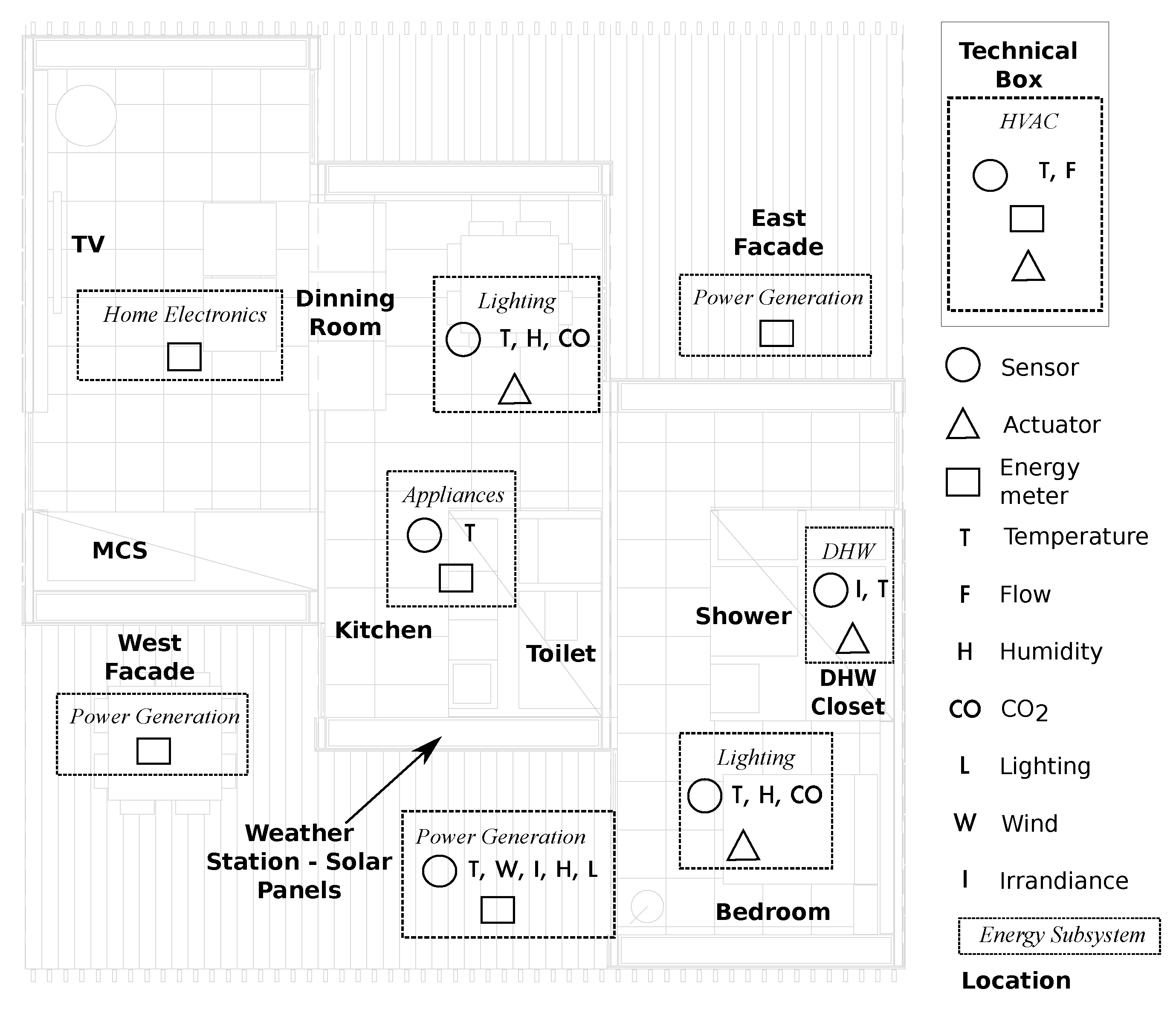
A sensor and control framework shown in Figure 1 has been used in the SMLsystem. It is operated by a Master Control Server (MCS) and the European home automation standard protocol known as Konnex (KNX) [19] has been chosen for monitoring and sensing. KNX modules are grouped by functionality: analog or binary inputs/outputs, gateways between transmission media, weather stations, CO${}_2$ detectors, etc. The whole system provides 88 sensor values and 49 actuators. In the proposed system, the immediate execution actions had been programmed to operate without the involvement of the MCS, such as controlling ventilation, the HVAC system and the DHW system. Beyond this basic level, the MCS can read the status of sensors and actuators at any time and can perform actions on them via an Ethernet gateway.

Figure 1. Small medium large system (SMLsystem) sensors and actuators map.

Figure 1. Small medium large system (SMLsystem) sensors and actuators map.

A monitoring and control software was developed following a three-layered scheme. In the first layer, data is acquired from the KNX bus using a KNX-IP (Internet Protocol) bridge device. The Open Home Automation Bus (openHAB) [20] software performs the communication between KNX and our software. In the second layer, it is possible to find a data persistence module that has been developed to collect the values offered by openHAB with a sampling period of 60 s. Finally, the third layer is composed of different software applications that are able to intercommunicate: a mobile application has been developed to let the user watch and control the current state of domotic devices; and different intelligence modules are being developed also, for instance, the ANN-based indoor temperature forecasting module.

The energy power generation systems described previously are monitored by a software controller. It includes multiple measurement sensors, including the voltage and current measurements of photovoltaic panels and batteries. Furthermore, the current, voltage and power of the grid is available. The system power consumption of the house has sensors for measuring power energy values for each group element. The climate system has power consumption sensors for the whole system, and specifically for the heat pump. The HVAC system is composed of several actuators and sensors used for operation. Among them are the inlet and outlet temperatures of the heat rejector and the inlet and outlet temperatures of the HVAC water in the SMLsystem. In addition, there are fourteen switches for internal function valves, for the fan coil system, for the heat pump and the heat rejector. The DHW system uses a valve and a pump to control water temperature. Some appliances have temperature sensors which are also monitored. The lighting system has sixteen binary actuators that can be operated manually by using the wall-mounted switches or by the MCS. The SMLsystem has indoor sensors for temperature, humidity and CO${}_2$. Outdoor sensors are also available for lighting measurements, wind speed, rain, irradiance and temperature.

3. Time Series Forecasting

Forecasting techniques are useful in terms of energy efficiency, because they help to develop predictive control systems. This section introduces formal aspects and forecasting modeling done for this work. Time series are data series with trend and pattern repetition through time. They can be formalized as a sequence of scalars from a variable x, obtained as the output of the observed process:

$$\overline{s}\left(x\right)=s_0\left(x\right),s_1\left(x\right),\dots ,s_{i-1}\left(x\right),s_i\left(x\right),s_{i+1}\left(x\right)$$

(1)

a fragment beginning at position i and ending at position j will be denoted by $s_i^j\left(x\right)$.

Time series forecasting could be grouped as univariate forecasting when the system forecasts variable x using only past values of x, and multivariate forecasting when the system forecasts variable x using past values of x plus additional values of other variables. Multivariate approaches could perform better than univariate when additional variables cause variations on the predicted variable x, as is shown in the experimental section.

Forecasting models are estimated given different parameters: the number of past values, the size of the future window, and the position in the future of the prediction (future horizon). Depending on the size of the future window and how it is produced [21], forecasting approaches are denoted as: single-step-ahead forecasting if the model forecasts only the next time step; multi-step-ahead iterative forecasting if the model forecasts only the next time step, producing longer windows by an iterative process; and multi-step-ahead direct forecasting [22] if the model forecasts in one step a large future window of size Z. Following this last approach, two different major model types exist:

• Pure direct, which uses Z forecasting models, one for each possible future horizon.
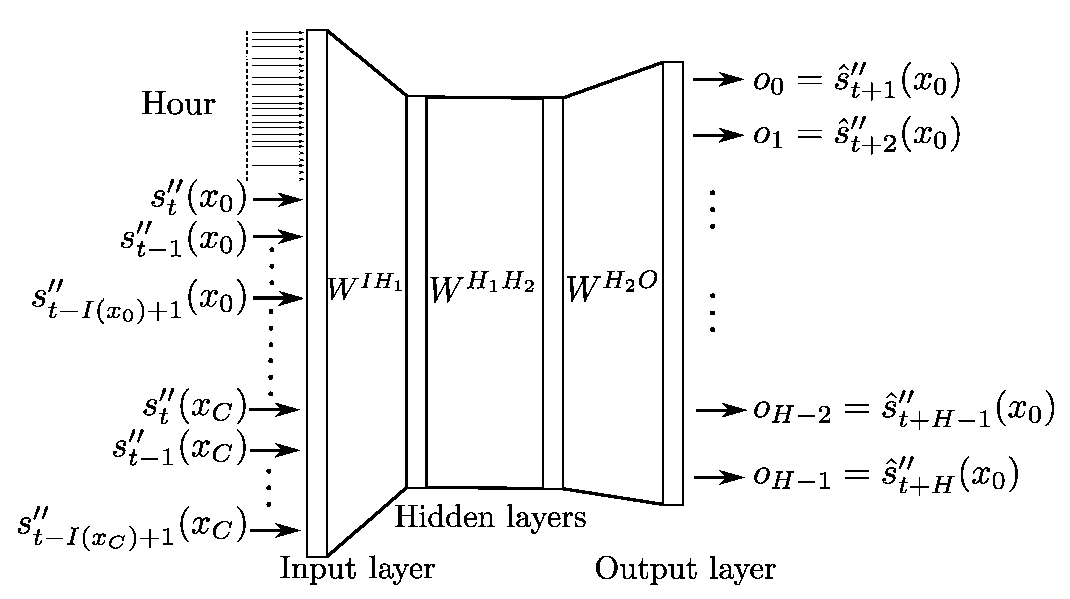
• Multiple input multiple output (MIMO), which uses one model to compute the full Z future window. This approach has several advantages due to the joint learning of inputs and outputs, which allows the model to learn the stochastic dependency between predicted values. Discriminative models, as ANNs, profit greatly from this input/output mapping. Additionally, ANNs are able to learn non-linear dependencies.

3.1. Forecast Model Formalization

A forecast model could be formalized as a function F, which receives as inputs the interest variable ($x_0$) with its past values until current time t and a number C of covariates ($x_1,x_2,\dots ,x_C$), also with its past values, until current time t and produces a future window of size Z for the given $x_0$ variable:

$$\langle {\widehat{s}}_{t+1}\left(x_0\right),{\widehat{s}}_{t+2}\left(x_0\right),\dots ,{\widehat{s}}_{t+Z}\left(x_0\right)\rangle =F(\mathsf{\Omega }\left(x_0\right),\mathsf{\Omega }\left(x_1\right),\dots ,\mathsf{\Omega }\left(x_C\right))$$

(2)

$\mathsf{\Omega }\left(x\right)=s_{t-I\left(x\right)+1}^t\left(x\right)$ being the $I\left(x\right)$ past values of variable/covariate x.

The number of past values $I\left(x\right)$ is important to ensure good performance of the model, however, it is not easy to estimate this number exactly. In this work, it is proposed to estimate models for several values of $I\left(x\right)$ and use the model that achieves better performance, denoted as BEST. It is known in the machine learning community that ensemble methods achieve better generalization [23,24,25]. Several possibilities could be found in the literature, such as vote combination, linear combination (for which a special case is the uniform or mean combination), or in a more complicated way, modular neural networks [26]. Hence, it is also proposed to combine the outputs of all estimated models for each different value of $I\left(x\right)$, following a linear combination scheme (the linear combination is also known as ensemble averaging), which is a simple, but effective method of combination, greatly extended to the machine learning community. Its major benefit is the reduction of overfitting problems and therefore, it could achieve better performance than a unique ANN. The quality of the combination depends on the correlation of the ANNs, theoretically, as the more decorrelated the models are, the better the combination is. In this way, different input size $I\left(x\right)$ ANNs were combined, with the expectation that they will be less correlated between themselves than other kinds of combinations, as modifying hidden layer size or other hyper-parameters.

A linear combination of forecasts models, given a set $F_{{\theta }_1},F_{{\theta }_2},\dots ,F_{{\theta }_M}$ of M forecast models, with the same future window size (Z), follows this equation:

$$\langle {\widehat{s}}_{t+1}\left(x_0\right),{\widehat{s}}_{t+2}\left(x_0\right),\dots ,{\widehat{s}}_{t+Z}\left(x_0\right)\rangle =\sum _{i=1}^M{\alpha }_i{F}_{{\theta }_i}({\mathsf{\Omega }}_i\left(x_0\right),{\mathsf{\Omega }}_i\left(x_1\right),\dots ,{\mathsf{\Omega }}_i\left(x_C\right))$$

(3)

where ${\alpha }_i$ is the combination weight given to the model ${\theta }_i$; and ${\mathsf{\Omega }}_i\left(x\right)$ is its corresponding Ω function, as described in Section 3.1. The weights are constrained to sum one, ${\sum }_{i=1}^M{\alpha }_i=1$. This formulation allows one to combine forecast models with different input window sizes for each covariate, but all of them using the same covariate inputs. Each weight ${\alpha }_i$ will be estimated following two approaches:

• Uniform linear combination: ${\alpha }_i=\frac{1}{M}$ for $1\le i\le M$. Models following this approach will be denoted as COMB-EQ.
• Exponential linear combination (softmax):

  $${\alpha }_i=\frac{exp\left(L^{-1}({\theta }_i,\mathcal{D})\right)}{{\sum }_{i=1}^{M}exp\left(L^{-1}({\theta }_i,\mathcal{D})\right)}$$

  (4)

  for $1\le i\le M$, $L^{-1}({\theta }_i,\mathcal{D})=1/L({\theta }_i,\mathcal{D})$ being an inverted loss-function (error function) value for the model ${\theta }_i$, given the dataset $\mathcal{D}$. It will be computed using a validation dataset. In this paper, the loss-function will be the mean absolute error (MAE), defined in Section 3.2, because it is more robust on outlier errors than other quadratic error measures. This approach will be denoted as COMB-EXP.

3.2. Evaluation Measures

The performance of forecasting methods over one time series could be assessed by several different evaluation functions, which measure the empirical error of the model. In this work, for a deep analysis of the results, three different error functions are used: MAE, root mean square error (RMSE) and symmetric mean absolute percentage of error (SMAPE). The error is computed comparing target values for the time series $s_{t+1},s_{t+2},\dots ,s_{t+Z}$, and its corresponding time series prediction ${\widehat{s}}_{t+1},{\widehat{s}}_{t+2},\dots ,{\widehat{s}}_{t+Z}$, using the model ${\theta }_{}$:

$$\begin{array}{ccc}\hfill \text{MAE}({\theta }_{},t)& =& \frac{1}{Z}\sum _{z=1}^Z|{\widehat{s}}_{t+z}\left(x_0\right)-s_{t+z}\left(x_0\right)|\hfill \end{array}$$

(5)

$$\begin{array}{ccc}\hfill \text{RMSE}({\theta }_{},t)& =& \sqrt{\frac{1}{Z}\sum _{z=1}^Z{({\widehat{s}}_{t+z}\left(x_0\right)-s_{t+z}\left(x_0\right))}^2}\hfill \end{array}$$

(6)

$$\begin{array}{ccc}\hfill \text{SMAPE}({\theta }_{},t)& =& \frac{1}{Z}\sum _{z=1}^Z\frac{|{\widehat{s}}_{t+z}-s_{t+z}|}{\left(\right|{\widehat{s}}_{t+z}|+|s_{t+z}\left|\right)/2}\times 100\hfill \end{array}$$

(7)

The results could be measured over all time series in a given dataset $\mathcal{D}$ as:

$$L^{*}({\theta }_{},\mathcal{D})=\frac{1}{\left|\mathcal{D}\right|}\sum _{t=1}^{\left|\mathcal{D}\right|}L({\theta }_{},t)$$

(8)

$\left|\mathcal{D}\right|$ being the size of the dataset and $L=\{\text{MAE},\text{RMSE},\text{SMAPE}\}$, the loss-function defining MAE${}^{*}$, RMSE${}^{*}$, and SMAPE${}^{*}$.

3.3. Forecasting Data Description

One aim of this work is to compare different statistical methods to forecast indoor temperature given previous indoor temperature values. The correlation between different weather signals and indoor temperature will also be analyzed.

In our database, time series are measured with a sampling period of $T=1$ min. However, in order to compute better forecasting models, each time series is sub-sampled with a period of $T^{\prime }=15$ min, computing the mean of the last $T^{\prime }$ values (for each hour, this mean is computed at 0 min, 15 min, 30 min and 45 min). The output of this preprocessing is the data series $s^{\prime }\left(x\right)$, where:

$${\displaystyle s_i^{\prime }\left(x\right)=\frac{{\displaystyle \sum _{j=(i-1)T^{\prime }+1}^{i{T}^{\prime }}{s}_j\left(x\right)}}{T^{\prime }}}$$

(9)

One time feature and five sensor signals were taken into consideration:

• Indoor temperature in degrees Celsius, denoted by variable $x=d$. This is the interesting forecasted variable.
• Hour feature in Universal Time Coordinated (UTC), extracted from the time-stamp of each pattern, denoted by variable $x=h$. The hour of the day is important for estimating the Sun’s position.
• Sun irradiance in $W/m^2$, denoted by variable $x=W$. It is correlated with temperature, because more irradiance will mean more heat.
• Indoor relative humidity percentage, denoted by variable $x=H$. The humidity modifies the inertia of the temperature.
• Indoor air quality in CO${}_2$ ppm (parts per million), denoted by variable $x=Q$. The air quality is related to the number of persons in the house, and a higher number of persons means an increase in temperature.
• Raining Boolean status, denoted by variable $x=R$. The result of sub-sampling this variable is the proportion of minutes in sub-sampling period $T^{\prime }$, where raining sensor was activated with True.

To evaluate the forecasting models’ performance, three partitions of our dataset were prepared: a training partition composed of 2017 time series over 21 days—the model parameters are estimated to reduce the error in this data; a validation partition composed of 672 time series over seven days—this is needed to avoid over-fitting during training, and also to compare and study the models between themselves; training and validation were performed in March 2011; a test partition composed of 672 time series over seven days in June 2011. At the end, the forecasting error in this partition will be provided, evaluating the generalization ability of this methodology. The validation partition is sequential with the training partition. The test partition is one week ahead of the last validation point.

4. Forecasting Methods

4.1. Standard Statistical Methods

Exponential smoothing and auto-regressive integrated moving average models (ARIMA) are the two most widely-used methods for time series forecasting. These methods provide complementary approaches to the time series forecasting problems. Therefore, exponential smoothing models are based on a description of trend and seasonality in the data, while ARIMA models aim to describe its autocorrelations. Their results have been considered as a reference to compare to the ANN results.

On the one hand, exponential smoothing methods are applied for forecasting. These methods were originally classified by [27] according to their taxonomy. This was later extended by [28], modified by [29] and extended by [30], giving a total of fifteen methods. These methods could have different behavior depending on their error component [A (additive) and M (multiplicative)], trend component [N (none), A (additive), Ad (additive damped), M (multiplicative) and Md (multiplicative damped)] and seasonal component [N (none), A (additive) and M (multiplicative)]. To select the best-fitting models within this framework, each possible model was estimated for the training partition, and the two best models were selected. To carry out this selection, Akaike’s Information Criterion (AIC) was used as suggested by some works in the literature [31,32]. The selected models were: the first model with multiplicative error, multiplicative damped trend and without the seasonal component (MMdN model), and the second model with additive error, additive damped trend and without the seasonal component (AAdN model). The MMdN model was chosen for the validation partition in order to minimize the MSE.

On the other hand, ARIMA models were estimated. The widely known ARIMA approach was first introduced by Box and Jenkins [33] and provides a comprehensive set of tools for univariate time series modeling and forecasting. These models were estimated for our data with and without covariates. The last value of variable hour ($x=h$), codified as a factor—using 24 categories (0 to 23), —and the hour as a continuous variable were used as covariates.

Either linear and quadratic form of this quantity were used, but linear performs worst. Therefore, three model groups are used: ARIMA without covariates (ARIMA), with covariate $x=h$ as a factor (ARIMAF) and with covariate $x=h$ as a quadratic form (ARIMAQ). The best models for each group were estimated for the training partition, and in all cases, the non-seasonal ARIMA(2,1,0) model was selected for the ARIMA part of each model using AIC. The best results, in terms of MSE, were obtained in models with covariate time as a factor and covariate time as a quadratic form.

The forecast library in the statistical package R [34] was used for these analyses.

4.2. ANNs

Estimation of ANN forecast models needs data preprocessing and normalization of input/output values in order to ensure better performance results.

4.2.1. Preprocessing of Time Series for ANNs

The indoor temperature variable ($x=d$) is the interesting forecasted variable. In order to increase model generalization, this variable is differentiated, and a new ${\overline{s}}^{″}(x=d)$ signal sequence is obtained following this equation:

$$s_i^{″}(x=d)=s_i^{\prime }\left(x\right)-s_{i-1}^{\prime }\left(x\right)$$

(10)

The differentiation of indoor temperature shows that is important to achieve good generalization results, and it is based on previous work where undifferentiated data has been used [11].

The time series corresponding to sun irradiance ($x=W$), indoor relative humidity ($x=H$), air quality ($x=Q$) and rain ($x=R$) are normalized, subtracting the mean and dividing by the standard deviation, computing new signal sequences, ${\overline{s}}^{″}(x\in \{W,H,Q,R\})$:

$${\displaystyle s_i^{″}(x\in \{W,H,Q,R\})=\frac{s_i^{\prime }\left(x\right)-\mathbb{E}\left[{\overline{s}}^{\prime }\left(x\right)\right]}{\sigma \left({\overline{s}}^{\prime }\left(x\right)\right)}}$$

(11)

where $\mathbb{E}\left[{\overline{s}}^{\prime }\left(x\right)\right]$ is the mean value of the sequence; ${\overline{s}}^{\prime }\left(x\right)$ and $\sigma \left({\overline{s}}^{\prime }\left(x\right)\right)$ is the standard deviation. These two parameters may be computed over the training dataset. For the hour component ($x=h$), a different approach is followed. It is represented as a locally-encoded category, which consists of using a vector with 24 components, where 23 components are set to 0, and the component that indicates the hour value is set to 1. This kind of encoding avoids the big jump between 23 and 0 at midnight, but forces the model to learn the relationship between adjacent hours. Other approaches for hour encoding could be done in future work.

4.2.2. ANN Description

ANNs has an impressive ability to learn complex mapping functions, as they are universal function approximators [35] and are widely used in forecasting [10,25,36,37].

ANNs are formed by one input layer, an output layer, and a few numbers of hidden layers. Figure 2 is a schematic representation of an ANN with two hidden layers for time series forecasting. The inputs of the ANN are past values of covariates, and the output layer is formed by the Z future window predicted values, following the MIMO approach described in Section 3, which has obtained better accuracy in previous experimentation [11].

Figure 2. Artificial neural network (ANN) topology for time series forecasting.

Figure 2. Artificial neural network (ANN) topology for time series forecasting.

The well-known error-backpropagation (BP) algorithm [38] has been used in its on-line version to estimate the ANN weights, adding a momentum term and an L2 regularization term (weight decay). Despite that theoretically algorithms more advanced than BP exists nowadays, BP is easier to implement at the empirical level, and a correct adjustment of momentum and weight decay helps to avoid bad local minima. The BP minimizes the mean square error (MSE) function with the addition of the regularization term weight decay, denoted by ϵ, useful for avoiding over-fitting and improving generalization:

$${\displaystyle E=\frac{1}{2Z}\sum _{i=1}^Z{\left({\widehat{s}}_{t+i}\left(x_0\right)-s_{t+i}\left(x_0\right)\right)}^2+\frac{ϵ}{2}\sum _{w_i\in {\theta }_{}}{w}_i^2}$$

(12)

where ${\theta }_{}$ is a set of all weights of the ANN (without the bias); and $w_i$ is the value of the i-th weight.

5. Experimental Results

Using the data acquired during the normal functioning of the house, experiments were performed to obtain the best forecasting model for indoor temperature. First, an exhaustive search of model hyper-parameters was done for each covariate combination. Second, different models were trained for different values of past size for indoor temperature $(x=d)$, and a comparison among different covariate combinations and ANN vs. standard statistical methods has been performed. A comparison of a combination of forecasting models has also been performed. In all cases, the future window size Z was set to 12, corresponding to a three-hour forecast.

A grid search exploration was done to set the best hyper-parameters of the system and ANN topology, fixing covariates $x\in \{d,W,H,Q,R\}$ to a past size, $I\left(x\right)=5$ and $I(x=h)=1$, searching combinations of:

• different covariates of the model input;
• different values for ANN hidden layer sizes;
• learning rate, momentum term and weight decay values.

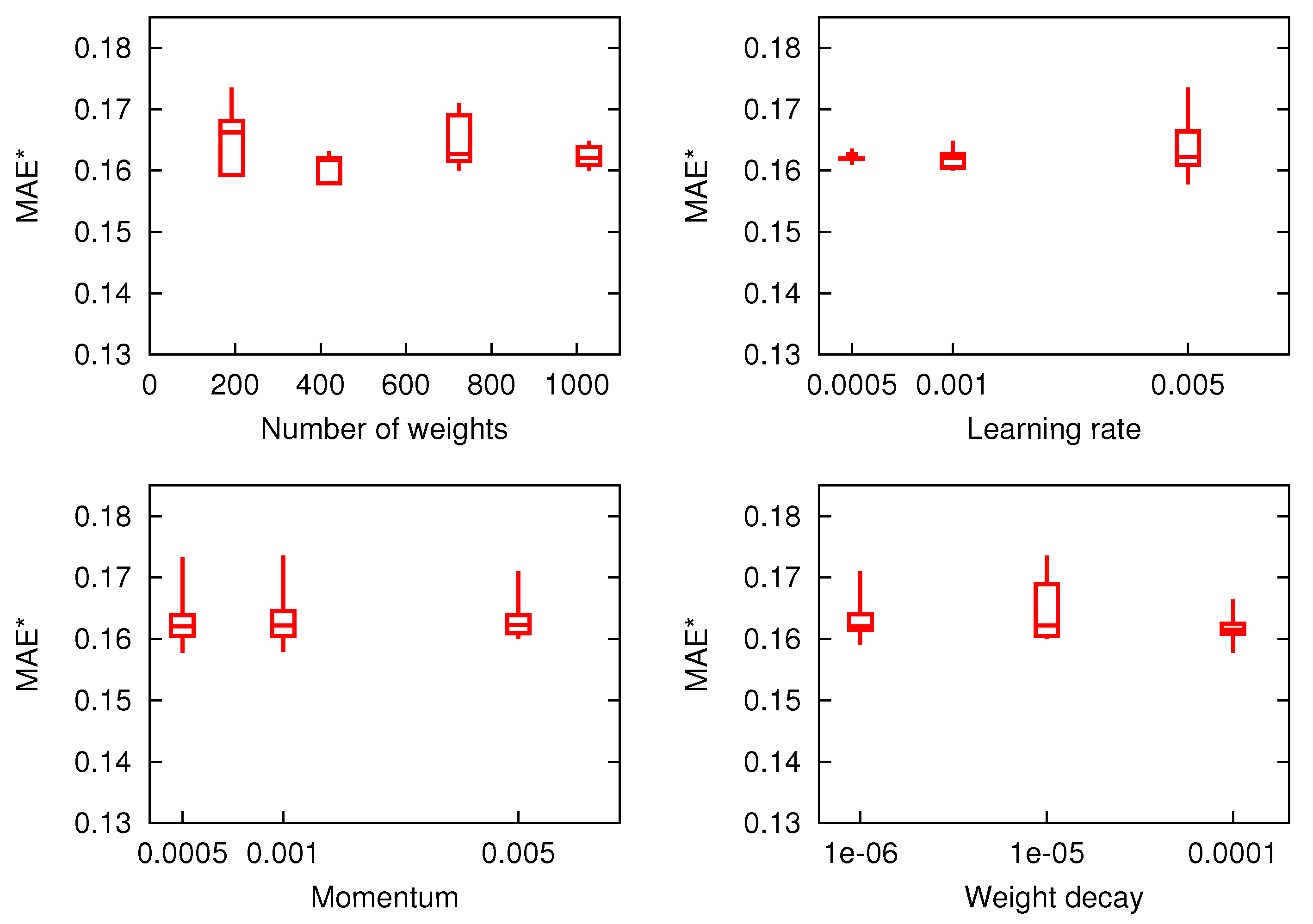
Table 2 shows the best model parameters found by this grid search. For illustrative purposes, Figure 3 and Figure 4 show box-and-whisker plots of the hyper-parameter grid search performed to optimize the ANN model, $d+h$.

Table 2. Training parameters depending on the input covariates combination (η is the learning rate, μ is the momentum term, and ϵ is weight decay).

Covariates	η	μ	ϵ	Hidden layers
d	$0.005\phantom{0}$	$0.001$	$1\times {10}^{-6}$	8 tanh–8 tanh
$d+W$	$0.001\phantom{0}$	$0.005$	$1\times {10}^{-6}$	24 tanh–8 tanh
$d+h$	$0.005\phantom{0}$	$0.005$	$1\times {10}^{-6}$	8 tanh
$d+h+W$	$0.005\phantom{0}$	$0.005$	$1\times {10}^{-5}$	24 tanh–16 tanh
$d+h+H$	$0.005\phantom{0}$	$0.005$	$1\times {10}^{-5}$	16 tanh
$d+h+R$	$0.005\phantom{0}$	$0.005$	$1\times {10}^{-6}$	16 logistic–8 logistic
$d+h+Q$	$0.0005$	$0.005$	$1\times {10}^{-4}$	24 logistic
$d+h+W+H$	$0.005\phantom{0}$	$0.005$	$1\times {10}^{-5}$	16 tanh
$d+h+W+R$	$0.005\phantom{0}$	$0.005$	$1\times {10}^{-6}$	16 logistic–8 logistic
$d+h+W+Q$	$0.005\phantom{0}$	$0.005$	$1\times {10}^{-4}$	8 tanh–8 tanh
$d+h+W+Q+R$	$0.005\phantom{0}$	$0.005$	$1\times {10}^{-4}$	24 tanh–8 tanh

Table 2. Training parameters depending on the input covariates combination (η is the learning rate, μ is the momentum term, and ϵ is weight decay).

Covariates	η	μ	ϵ	Hidden layers
d	$0.005\phantom{0}$	$0.001$	$1\times {10}^{-6}$	8 tanh–8 tanh
$d+W$	$0.001\phantom{0}$	$0.005$	$1\times {10}^{-6}$	24 tanh–8 tanh
$d+h$	$0.005\phantom{0}$	$0.005$	$1\times {10}^{-6}$	8 tanh
$d+h+W$	$0.005\phantom{0}$	$0.005$	$1\times {10}^{-5}$	24 tanh–16 tanh
$d+h+H$	$0.005\phantom{0}$	$0.005$	$1\times {10}^{-5}$	16 tanh
$d+h+R$	$0.005\phantom{0}$	$0.005$	$1\times {10}^{-6}$	16 logistic–8 logistic
$d+h+Q$	$0.0005$	$0.005$	$1\times {10}^{-4}$	24 logistic
$d+h+W+H$	$0.005\phantom{0}$	$0.005$	$1\times {10}^{-5}$	16 tanh
$d+h+W+R$	$0.005\phantom{0}$	$0.005$	$1\times {10}^{-6}$	16 logistic–8 logistic
$d+h+W+Q$	$0.005\phantom{0}$	$0.005$	$1\times {10}^{-4}$	8 tanh–8 tanh
$d+h+W+Q+R$	$0.005\phantom{0}$	$0.005$	$1\times {10}^{-4}$	24 tanh–8 tanh

Figure 3. Mean absolute error (MAE)${}^{*}$ box-and-whisker plots for ANNs with one hidden layer and the hyper-parameters of the grid search performed to optimize the ANN model, $d+h$. The x-axis of the learning rate, momentum and weight decay are log-scaled.

Figure 3. Mean absolute error (MAE)${}^{*}$ box-and-whisker plots for ANNs with one hidden layer and the hyper-parameters of the grid search performed to optimize the ANN model, $d+h$. The x-axis of the learning rate, momentum and weight decay are log-scaled.

Figure 4. MAE${}^{*}$ box-and-whisker plots for ANNs with two hidden layers and the hyper-parameters of the grid search performed to optimize the ANN model, $d+h$. The x-axis of the learning rate, momentum and weight decay are log-scaled.

Figure 4. MAE${}^{*}$ box-and-whisker plots for ANNs with two hidden layers and the hyper-parameters of the grid search performed to optimize the ANN model, $d+h$. The x-axis of the learning rate, momentum and weight decay are log-scaled.

They show big differences between one- and two-hidden layer ANNs, two-layered ANNs being more difficult to train for this particular model. The learning rate shows a big impact in performance, while momentum and weight decay seems to be less important. This grid search was repeated for all the tested covariate combinations, and the hyper-parameters that optimize MAE${}^{*}$ were selected in the rest of the paper.

5.1. Covariate Analysis and Comparison between Different Forecasting Strategies

For each covariate combination, and using the best model parameters obtained previously, different model comparison has been performed. Note that the input past size of covariates is set to $I(x\in \{W,H,Q,R\left\}\right)$= 5 time steps, that is, 60 min, and to $I(x=h)=1$. For forecasted variable $x=d$, models with sizes $I(x=d)\in \{1,3,5,7,9,11,13,15,17,19,21\}$ were trained.

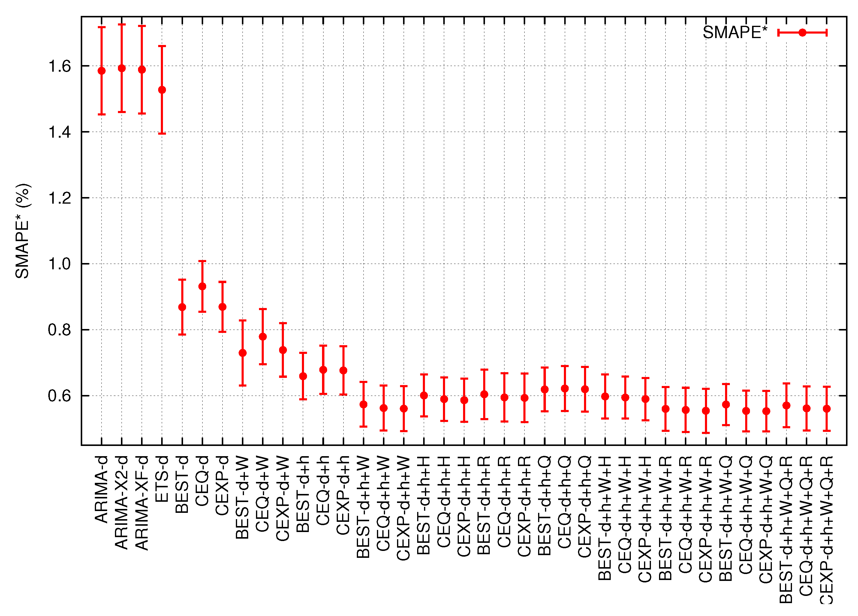
A comparison between BEST, COMB-EQ and COMB-EXP approaches was performed and shown in Table 3. Figure 5 plots the same results for a better confidence interval comparison. Table 4 shows COMB-EQ weights used in experimentation, obtained following Equation (4) and using MAE${}^{*}$ as the loss-function. From all these results, the superiority of ANNs vs. standard statistical methods is clear, with clear statistical significance and with a confidence greater than $99\%$. Different covariate combinations for ANN models show that the indoor temperature correlates well with the hour ($d+h$) and sun irradiance ($d+W$), and the combination of these two covariates ($d+h+W$) improves the model in a significant way ($99\%$ confidence) with input $d+W$. The addition of more covariates is slightly better in two cases ($d+h+W+R$ and $d+h+W+Q$), but the differences are not important. With only the hour and sun irradiance, the ANN model has enough information to perform good forecasting. Regarding the combination of models, in some cases, the COMB-EXP approach obtains consistently better results than COMB-EQ and BEST, but the differences are not important.

Table 3. Symmetric mean absolute percentage of error (SMAPE)${}^{*}$, MAE${}^{*}$ and root mean square error (RMSE)${}^{*}$ results on the validation partition comparing different models, input features and combination schemes with the $99\%$ confidence interval. BEST refers to the best past size ANN, CEQ refers to COMB-EQ ANNs, and CEXP refers to COMB-EXP ANNs. Bolded face numbers are the best results, and the gray marked row is the most significant combination of covariates. ARIMA: auto-regressive integrated moving average models; ARIMAQ: ARIMA with covariate $x=h$ as a quadratic form (ARIMAQ); ARIMAF: ARIMA with covariate $x=h$ as a factor.

Model	SMAPE ${}^{\mathbf{*}}(\%)[lower,upper]$			MAE${}^{\mathbf{*}}[lower,upper]$			RMSE${}^{\mathbf{*}}[lower,upper]$
Standard statistical models
ARIMA-d	$1.5856$	$[1.4528,$	$1.7183]$	$0.3099$	$[0.2851,$	$0.3348]$	$0.3715$	$[0.3413,$	$0.4016]$
ARIMAQ-$d+h^2$	$1.5932$	$[1.4607,$	$1.7257]$	$0.3113$	$[0.2865,$	$0.3362]$	$0.3729$	$[0.3428,$	$0.4029]$
ARIMAF-$d+h$	$1.5888$	$[1.4558,$	$1.7219]$	$0.3105$	$[0.2857,$	$0.3352]$	$0.3721$	$[0.3420,$	$0.4022]$
ETS-d	$1.5277$	$[1.3946,$	$1.6607]$	$0.3004$	$[0.2753,$	$0.3255]$	$0.3648$	$[0.3340,$	$0.3957]$
ANN models
BEST-d	$0.8687$	$[0.7856,$	$0.9517]$	$0.1682$	$[0.1524,$	$0.1840]$	$0.2109$	$[0.1911,$	$0.2306]$
CEQ-d	$0.9315$	$[0.8545,$	$1.0085]$	$0.1802$	$[0.1661,$	$0.1944]$	$0.2248$	$[0.2072,$	$0.2423]$
CEXP-d	$0.8695$	$[0.7938,$	$0.9452]$	$0.1680$	$[0.1541,$	$0.1818]$	$0.2109$	$[0.1937,$	$0.2280]$
BEST-$d+W$	$0.7296$	$[0.6311,$	$0.8281]$	$0.1418$	$[0.1228,$	$0.1608]$	$0.1777$	$[0.1544,$	$0.2010]$
CEQ-$d+W$	$0.7792$	$[0.6959,$	$0.8625]$	$0.1510$	$[0.1353,$	$0.1667]$	$0.1888$	$[0.1695,$	$0.2082]$
CEXP-$d+W$	$0.7387$	$[0.6576,$	$0.8199]$	$0.1430$	$[0.1277,$	$0.1582]$	$0.1788$	$[0.1601,$	$0.1975]$
BEST-$d+h$	$0.6593$	$[0.5889,$	$0.7298]$	$0.1275$	$[0.1143,$	$0.1406]$	$0.1549$	$[0.1389,$	$0.1708]$
CEQ-$d+h$	$0.6787$	$[0.6055,$	$0.7519]$	$0.1312$	$[0.1175,$	$0.1449]$	$0.1590$	$[0.1425,$	$0.1754]$
CEXP-$d+h$	$0.6768$	$[0.6037,$	$0.7498]$	$0.1308$	$[0.1172,$	$0.1445]$	$0.1586$	$[0.1422,$	$0.1750]$
BEST-$d+h+W$	$0.5737$	$[0.5058,$	$0.6416]$	$0.1121$	$[0.0994,$	$0.1248]$	$0.1379$	$[0.1222,$	$0.1536]$
CEQ-$d+h+W$	$0.5625$	$[0.4944,$	$0.6306]$	$0.1094$	$[0.0966,$	$0.1222]$	$0.1348$	$[0.1189,$	$0.1506]$
CEXP-$d+h+W$	$0.5608$	$[0.4927,$	$0.6289]$	$0.1091$	$[0.0963,$	$0.1218]$	$0.1344$	$[0.1187,$	$0.1501]$
BEST-$d+h+H$	$0.6006$	$[0.5369,$	$0.6642]$	$0.1169$	$[0.1050,$	$0.1288]$	$0.1429$	$[0.1285,$	$0.1573]$
CEQ-$d+h+H$	$0.5897$	$[0.5240,$	$0.6553]$	$0.1142$	$[0.1019,$	$0.1264]$	$0.1399$	$[0.1250,$	$0.1548]$
CEXP-$d+h+H$	$0.5864$	$[0.5207,$	$0.6521]$	$0.1137$	$[0.1014,$	$0.1259]$	$0.1393$	$[0.1244,$	$0.1543]$
BEST-$d+h+R$	$0.6042$	$[0.5292,$	$0.6792]$	$0.1170$	$[0.1031,$	$0.1309]$	$0.1424$	$[0.1255,$	$0.1593]$
CEQ-$d+h+R$	$0.5947$	$[0.5214,$	$0.6680]$	$0.1149$	$[0.1014,$	$0.1284]$	$0.1410$	$[0.1245,$	$0.1575]$
CEXP-$d+h+R$	$0.5933$	$[0.5196,$	$0.6670]$	$0.1146$	$[0.1009,$	$0.1282]$	$0.1407$	$[0.1241,$	$0.1574]$
BEST-$d+h+Q$	$0.6189$	$[0.5526,$	$0.6852]$	$0.1200$	$[0.1075,$	$0.1325]$	$0.1463$	$[0.1311,$	$0.1614]$
CEQ-$d+h+Q$	$0.6219$	$[0.5539,$	$0.6899]$	$0.1208$	$[0.1080,$	$0.1336]$	$0.1479$	$[0.1324,$	$0.1633]$
CEXP-$d+h+Q$	$0.6196$	$[0.5518,$	$0.6873]$	$0.1203$	$[0.1076,$	$0.1331]$	$0.1473$	$[0.1319,$	$0.1627]$
BEST-$d+h+W+H$	$0.5977$	$[0.5309,$	$0.6646]$	$0.1163$	$[0.1037,$	$0.1289]$	$0.1434$	$[0.1280,$	$0.1588]$
CEQ-$d+h+W+H$	$0.5943$	$[0.5304,$	$0.6583]$	$0.1155$	$[0.1034,$	$0.1275]$	$0.1424$	$[0.1276,$	$0.1571]$
CEXP-$d+h+W+H$	$0.5899$	$[0.5257,$	$0.6540]$	$0.1146$	$[0.1025,$	$0.1267]$	$0.1413$	$[0.1265,$	$0.1561]$
BEST-$d+h+W+R$	$0.5600$	$[0.4935,$	$0.6266]$	$0.1090$	$[0.0966,$	$0.1214]$	$0.1335$	$[0.1183,$	$0.1486]$
CEQ-$d+h+W+R$	$0.5568$	$[0.4895,$	$0.6240]$	$0.1080$	$[0.0955,$	$0.1205]$	$0.1328$	$[0.1174,$	$0.1482]$
CEXP-$d+h+W+R$	$0.5541$	$[0.4872,$	$0.6210]$	$\mathbf{0}.\mathbf{1076}$	$[0.0951,$	$0.1200]$	$\mathbf{0}.\mathbf{1323}$	$[0.1169,$	$0.1476]$
BEST-$d+h+W+Q$	$0.5732$	$[0.5111,$	$0.6353]$	$0.1118$	$[0.1000,$	$0.1236]$	$0.1376$	$[0.1231,$	$0.1521]$
CEQ-$d+h+W+Q$	$0.5537$	$[0.4921,$	$0.6153]$	$0.1079$	$[0.0962,$	$0.1196]$	$0.1328$	$[0.1184,$	$0.1472]$
CEXP-$d+h+W+Q$	$\mathbf{0}.\mathbf{5532}$	$[0.4916,$	$0.6148]$	$0.1079$	$[0.0962,$	$0.1196]$	$0.1328$	$[0.1184,$	$0.1472]$
BEST-$d+h+W+Q+R$	$0.5704$	$[0.5040,$	$0.6369]$	$0.1110$	$[0.0984,$	$0.1235]$	$0.1363$	$[0.1210,$	$0.1517]$
CEQ-$d+h+W+Q+R$	$0.5615$	$[0.4945,$	$0.6285]$	$0.1088$	$[0.0964,$	$0.1212]$	$0.1340$	$[0.1187,$	$0.1492]$
CEXP-$d+h+W+Q+R$	$0.5606$	$[0.4937,$	$0.6275]$	$0.1087$	$[0.0963,$	$0.1211]$	$0.1337$	$[0.1185,$	$0.1490]$

Table 3. Symmetric mean absolute percentage of error (SMAPE)${}^{*}$, MAE${}^{*}$ and root mean square error (RMSE)${}^{*}$ results on the validation partition comparing different models, input features and combination schemes with the $99\%$ confidence interval. BEST refers to the best past size ANN, CEQ refers to COMB-EQ ANNs, and CEXP refers to COMB-EXP ANNs. Bolded face numbers are the best results, and the gray marked row is the most significant combination of covariates. ARIMA: auto-regressive integrated moving average models; ARIMAQ: ARIMA with covariate $x=h$ as a quadratic form (ARIMAQ); ARIMAF: ARIMA with covariate $x=h$ as a factor.

Model	SMAPE ${}^{\mathbf{*}}(\%)[lower,upper]$			MAE${}^{\mathbf{*}}[lower,upper]$			RMSE${}^{\mathbf{*}}[lower,upper]$
Standard statistical models
ARIMA-d	$1.5856$	$[1.4528,$	$1.7183]$	$0.3099$	$[0.2851,$	$0.3348]$	$0.3715$	$[0.3413,$	$0.4016]$
ARIMAQ-$d+h^2$	$1.5932$	$[1.4607,$	$1.7257]$	$0.3113$	$[0.2865,$	$0.3362]$	$0.3729$	$[0.3428,$	$0.4029]$
ARIMAF-$d+h$	$1.5888$	$[1.4558,$	$1.7219]$	$0.3105$	$[0.2857,$	$0.3352]$	$0.3721$	$[0.3420,$	$0.4022]$
ETS-d	$1.5277$	$[1.3946,$	$1.6607]$	$0.3004$	$[0.2753,$	$0.3255]$	$0.3648$	$[0.3340,$	$0.3957]$
ANN models
BEST-d	$0.8687$	$[0.7856,$	$0.9517]$	$0.1682$	$[0.1524,$	$0.1840]$	$0.2109$	$[0.1911,$	$0.2306]$
CEQ-d	$0.9315$	$[0.8545,$	$1.0085]$	$0.1802$	$[0.1661,$	$0.1944]$	$0.2248$	$[0.2072,$	$0.2423]$
CEXP-d	$0.8695$	$[0.7938,$	$0.9452]$	$0.1680$	$[0.1541,$	$0.1818]$	$0.2109$	$[0.1937,$	$0.2280]$
BEST-$d+W$	$0.7296$	$[0.6311,$	$0.8281]$	$0.1418$	$[0.1228,$	$0.1608]$	$0.1777$	$[0.1544,$	$0.2010]$
CEQ-$d+W$	$0.7792$	$[0.6959,$	$0.8625]$	$0.1510$	$[0.1353,$	$0.1667]$	$0.1888$	$[0.1695,$	$0.2082]$
CEXP-$d+W$	$0.7387$	$[0.6576,$	$0.8199]$	$0.1430$	$[0.1277,$	$0.1582]$	$0.1788$	$[0.1601,$	$0.1975]$
BEST-$d+h$	$0.6593$	$[0.5889,$	$0.7298]$	$0.1275$	$[0.1143,$	$0.1406]$	$0.1549$	$[0.1389,$	$0.1708]$
CEQ-$d+h$	$0.6787$	$[0.6055,$	$0.7519]$	$0.1312$	$[0.1175,$	$0.1449]$	$0.1590$	$[0.1425,$	$0.1754]$
CEXP-$d+h$	$0.6768$	$[0.6037,$	$0.7498]$	$0.1308$	$[0.1172,$	$0.1445]$	$0.1586$	$[0.1422,$	$0.1750]$
BEST-$d+h+W$	$0.5737$	$[0.5058,$	$0.6416]$	$0.1121$	$[0.0994,$	$0.1248]$	$0.1379$	$[0.1222,$	$0.1536]$
CEQ-$d+h+W$	$0.5625$	$[0.4944,$	$0.6306]$	$0.1094$	$[0.0966,$	$0.1222]$	$0.1348$	$[0.1189,$	$0.1506]$
CEXP-$d+h+W$	$0.5608$	$[0.4927,$	$0.6289]$	$0.1091$	$[0.0963,$	$0.1218]$	$0.1344$	$[0.1187,$	$0.1501]$
BEST-$d+h+H$	$0.6006$	$[0.5369,$	$0.6642]$	$0.1169$	$[0.1050,$	$0.1288]$	$0.1429$	$[0.1285,$	$0.1573]$
CEQ-$d+h+H$	$0.5897$	$[0.5240,$	$0.6553]$	$0.1142$	$[0.1019,$	$0.1264]$	$0.1399$	$[0.1250,$	$0.1548]$
CEXP-$d+h+H$	$0.5864$	$[0.5207,$	$0.6521]$	$0.1137$	$[0.1014,$	$0.1259]$	$0.1393$	$[0.1244,$	$0.1543]$
BEST-$d+h+R$	$0.6042$	$[0.5292,$	$0.6792]$	$0.1170$	$[0.1031,$	$0.1309]$	$0.1424$	$[0.1255,$	$0.1593]$
CEQ-$d+h+R$	$0.5947$	$[0.5214,$	$0.6680]$	$0.1149$	$[0.1014,$	$0.1284]$	$0.1410$	$[0.1245,$	$0.1575]$
CEXP-$d+h+R$	$0.5933$	$[0.5196,$	$0.6670]$	$0.1146$	$[0.1009,$	$0.1282]$	$0.1407$	$[0.1241,$	$0.1574]$
BEST-$d+h+Q$	$0.6189$	$[0.5526,$	$0.6852]$	$0.1200$	$[0.1075,$	$0.1325]$	$0.1463$	$[0.1311,$	$0.1614]$
CEQ-$d+h+Q$	$0.6219$	$[0.5539,$	$0.6899]$	$0.1208$	$[0.1080,$	$0.1336]$	$0.1479$	$[0.1324,$	$0.1633]$
CEXP-$d+h+Q$	$0.6196$	$[0.5518,$	$0.6873]$	$0.1203$	$[0.1076,$	$0.1331]$	$0.1473$	$[0.1319,$	$0.1627]$
BEST-$d+h+W+H$	$0.5977$	$[0.5309,$	$0.6646]$	$0.1163$	$[0.1037,$	$0.1289]$	$0.1434$	$[0.1280,$	$0.1588]$
CEQ-$d+h+W+H$	$0.5943$	$[0.5304,$	$0.6583]$	$0.1155$	$[0.1034,$	$0.1275]$	$0.1424$	$[0.1276,$	$0.1571]$
CEXP-$d+h+W+H$	$0.5899$	$[0.5257,$	$0.6540]$	$0.1146$	$[0.1025,$	$0.1267]$	$0.1413$	$[0.1265,$	$0.1561]$
BEST-$d+h+W+R$	$0.5600$	$[0.4935,$	$0.6266]$	$0.1090$	$[0.0966,$	$0.1214]$	$0.1335$	$[0.1183,$	$0.1486]$
CEQ-$d+h+W+R$	$0.5568$	$[0.4895,$	$0.6240]$	$0.1080$	$[0.0955,$	$0.1205]$	$0.1328$	$[0.1174,$	$0.1482]$
CEXP-$d+h+W+R$	$0.5541$	$[0.4872,$	$0.6210]$	$\mathbf{0}.\mathbf{1076}$	$[0.0951,$	$0.1200]$	$\mathbf{0}.\mathbf{1323}$	$[0.1169,$	$0.1476]$
BEST-$d+h+W+Q$	$0.5732$	$[0.5111,$	$0.6353]$	$0.1118$	$[0.1000,$	$0.1236]$	$0.1376$	$[0.1231,$	$0.1521]$
CEQ-$d+h+W+Q$	$0.5537$	$[0.4921,$	$0.6153]$	$0.1079$	$[0.0962,$	$0.1196]$	$0.1328$	$[0.1184,$	$0.1472]$
CEXP-$d+h+W+Q$	$\mathbf{0}.\mathbf{5532}$	$[0.4916,$	$0.6148]$	$0.1079$	$[0.0962,$	$0.1196]$	$0.1328$	$[0.1184,$	$0.1472]$
BEST-$d+h+W+Q+R$	$0.5704$	$[0.5040,$	$0.6369]$	$0.1110$	$[0.0984,$	$0.1235]$	$0.1363$	$[0.1210,$	$0.1517]$
CEQ-$d+h+W+Q+R$	$0.5615$	$[0.4945,$	$0.6285]$	$0.1088$	$[0.0964,$	$0.1212]$	$0.1340$	$[0.1187,$	$0.1492]$
CEXP-$d+h+W+Q+R$	$0.5606$	$[0.4937,$	$0.6275]$	$0.1087$	$[0.0963,$	$0.1211]$	$0.1337$	$[0.1185,$	$0.1490]$

Figure 5. SMAPE${}^{*}$ error plot with $99\%$ confidence interval for models of Table 3 on the validation partition.

Figure 5. SMAPE${}^{*}$ error plot with $99\%$ confidence interval for models of Table 3 on the validation partition.

Table 4. Combination weights of every input size of d for the COMB-EXP models given tested covariates combinations. All co-variables have an input size of 5 (75 min). Bold numbers are the best input sizes.

Input covariates	COMB-EXP combination weights for every d variable input size (min)
	$1\left(15\right)$	$3\left(45\right)$	$5\left(75\right)$	$7\left(105\right)$	$9\left(135\right)$	$11\left(165\right)$	$13\left(195\right)$	$15\left(225\right)$	$17\left(255\right)$	$19\left(285\right)$	$21\left(315\right)$
d	$0.002$	$0.044$	$0.098$	$\mathbf{0}.\mathbf{142}$	$0.092$	$0.095$	$0.082$	$0.103$	$0.100$	$0.106$	$0.135$
$d+W$	$0.026$	$0.020$	$\mathbf{0}.\mathbf{185}$	$0.046$	$0.069$	$0.075$	$0.104$	$0.103$	$0.124$	$0.117$	$0.131$
$d+h$	$\mathbf{0}.\mathbf{123}$	$0.066$	$0.099$	$0.085$	$0.092$	$0.091$	$0.091$	$0.097$	$0.084$	$0.084$	$0.088$
$d+h+W$	$0.040$	$0.112$	$\mathbf{0}.\mathbf{137}$	$0.072$	$0.078$	$0.100$	$0.107$	$0.120$	$0.083$	$0.075$	$0.075$
$d+h+H$	$0.049$	$0.058$	$0.121$	$\mathbf{0}.\mathbf{127}$	$0.095$	$0.105$	$0.114$	$0.068$	$0.100$	$0.074$	$0.090$
$d+h+R$	$0.049$	$0.052$	$\mathbf{0}.\mathbf{126}$	$0.099$	$0.078$	$0.113$	$0.104$	$0.114$	$0.102$	$0.089$	$0.076$
$d+h+Q$	$0.084$	$0.089$	$0.105$	$\mathbf{0}.\mathbf{123}$	$0.115$	$0.103$	$0.086$	$0.077$	$0.069$	$0.073$	$0.076$
$d+h+W+H$	$0.062$	$0.085$	$0.071$	$0.091$	$0.123$	$\mathbf{0}.\mathbf{134}$	$0.094$	$0.082$	$0.067$	$0.121$	$0.069$
$d+h+W+R$	$0.048$	$0.089$	$\mathbf{0}.\mathbf{142}$	$0.078$	$0.062$	$0.116$	$0.121$	$0.092$	$0.109$	$0.087$	$0.056$
$d+h+W+Q$	$0.064$	$0.101$	$0.112$	$0.097$	$0.068$	$0.088$	$\mathbf{0}.\mathbf{115}$	$0.090$	$0.085$	$0.079$	$0.101$
$d+h+W+Q+R$	$0.042$	$0.090$	$\mathbf{0}.\mathbf{136}$	$0.098$	$0.111$	$0.089$	$0.101$	$0.072$	$0.090$	$0.085$	$0.087$

Table 4. Combination weights of every input size of d for the COMB-EXP models given tested covariates combinations. All co-variables have an input size of 5 (75 min). Bold numbers are the best input sizes.

Input covariates	COMB-EXP combination weights for every d variable input size (min)
	$1\left(15\right)$	$3\left(45\right)$	$5\left(75\right)$	$7\left(105\right)$	$9\left(135\right)$	$11\left(165\right)$	$13\left(195\right)$	$15\left(225\right)$	$17\left(255\right)$	$19\left(285\right)$	$21\left(315\right)$
d	$0.002$	$0.044$	$0.098$	$\mathbf{0}.\mathbf{142}$	$0.092$	$0.095$	$0.082$	$0.103$	$0.100$	$0.106$	$0.135$
$d+W$	$0.026$	$0.020$	$\mathbf{0}.\mathbf{185}$	$0.046$	$0.069$	$0.075$	$0.104$	$0.103$	$0.124$	$0.117$	$0.131$
$d+h$	$\mathbf{0}.\mathbf{123}$	$0.066$	$0.099$	$0.085$	$0.092$	$0.091$	$0.091$	$0.097$	$0.084$	$0.084$	$0.088$
$d+h+W$	$0.040$	$0.112$	$\mathbf{0}.\mathbf{137}$	$0.072$	$0.078$	$0.100$	$0.107$	$0.120$	$0.083$	$0.075$	$0.075$
$d+h+H$	$0.049$	$0.058$	$0.121$	$\mathbf{0}.\mathbf{127}$	$0.095$	$0.105$	$0.114$	$0.068$	$0.100$	$0.074$	$0.090$
$d+h+R$	$0.049$	$0.052$	$\mathbf{0}.\mathbf{126}$	$0.099$	$0.078$	$0.113$	$0.104$	$0.114$	$0.102$	$0.089$	$0.076$
$d+h+Q$	$0.084$	$0.089$	$0.105$	$\mathbf{0}.\mathbf{123}$	$0.115$	$0.103$	$0.086$	$0.077$	$0.069$	$0.073$	$0.076$
$d+h+W+H$	$0.062$	$0.085$	$0.071$	$0.091$	$0.123$	$\mathbf{0}.\mathbf{134}$	$0.094$	$0.082$	$0.067$	$0.121$	$0.069$
$d+h+W+R$	$0.048$	$0.089$	$\mathbf{0}.\mathbf{142}$	$0.078$	$0.062$	$0.116$	$0.121$	$0.092$	$0.109$	$0.087$	$0.056$
$d+h+W+Q$	$0.064$	$0.101$	$0.112$	$0.097$	$0.068$	$0.088$	$\mathbf{0}.\mathbf{115}$	$0.090$	$0.085$	$0.079$	$0.101$
$d+h+W+Q+R$	$0.042$	$0.090$	$\mathbf{0}.\mathbf{136}$	$0.098$	$0.111$	$0.089$	$0.101$	$0.072$	$0.090$	$0.085$	$0.087$

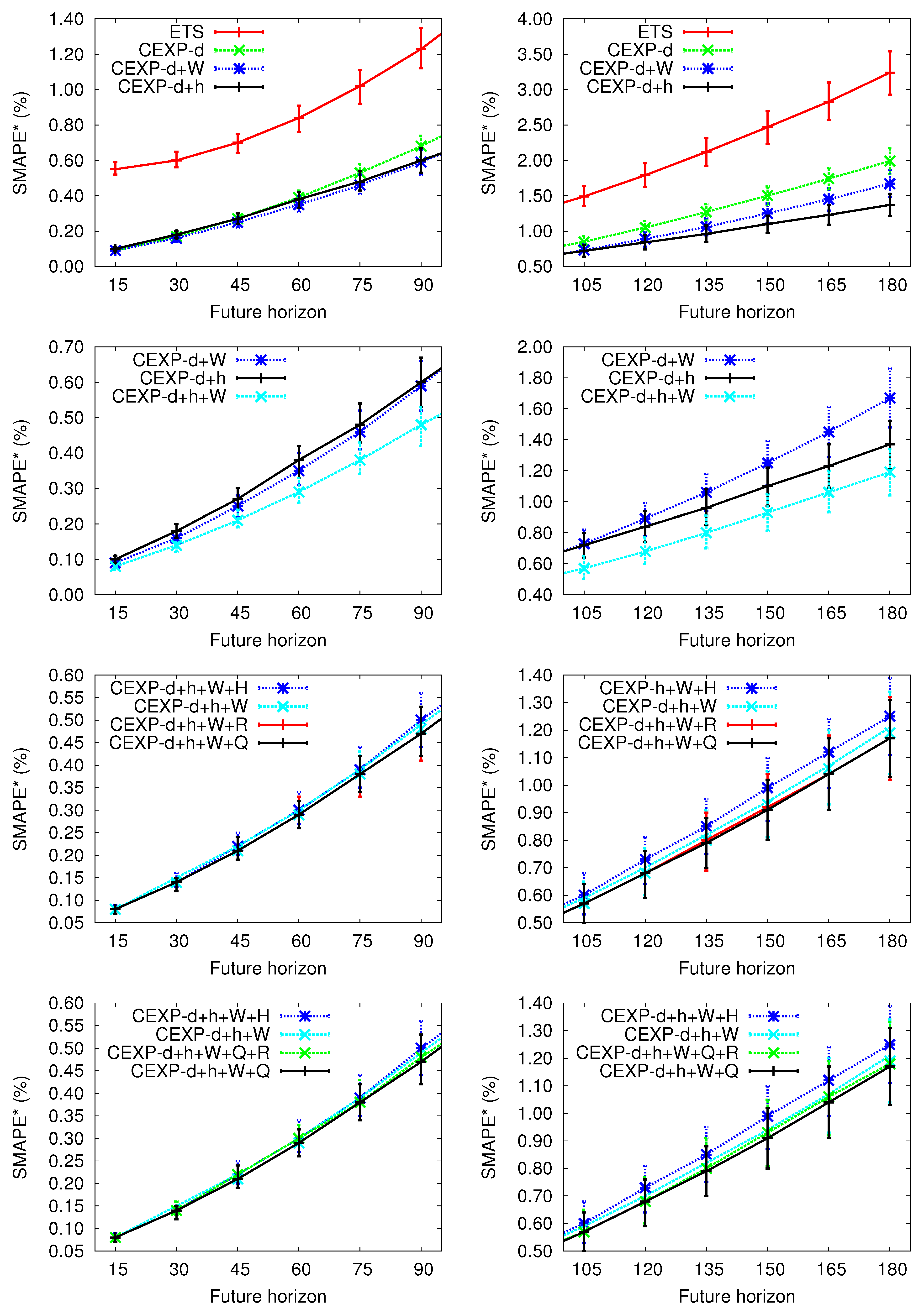
A deeper analysis could be done if comparing the SMAPE values for each possible future horizon, as Figure 6 shows. A clear trend exists: error increases with the enlargement of the future horizon. Furthermore, an enlargement of the confidence interval is observed with the enlargement of the future horizon. In all cases, ANN models outperform statistical methods. For shorter horizons (less than or equal to 90 min), the differences between all ANN models are insignificant. For longer horizons (greater than 90 min), a combination of covariates $d+h+W$ achieve a significant result (for a confidence of $99\%$) compared with the $d+W$ combination. As was shown in these results, the addition of covariates is useful when the future horizon increases, probably because the impact of covariates into indoor temperature becomes stronger over time.

Figure 6. SMAPE${}^{*}$ error plot with $99\%$ confidence interval of each of the $Z=12$ future horizon predicted values (from 15 min forecast to 180 min forecast.)

Figure 6. SMAPE${}^{*}$ error plot with $99\%$ confidence interval of each of the $Z=12$ future horizon predicted values (from 15 min forecast to 180 min forecast.)

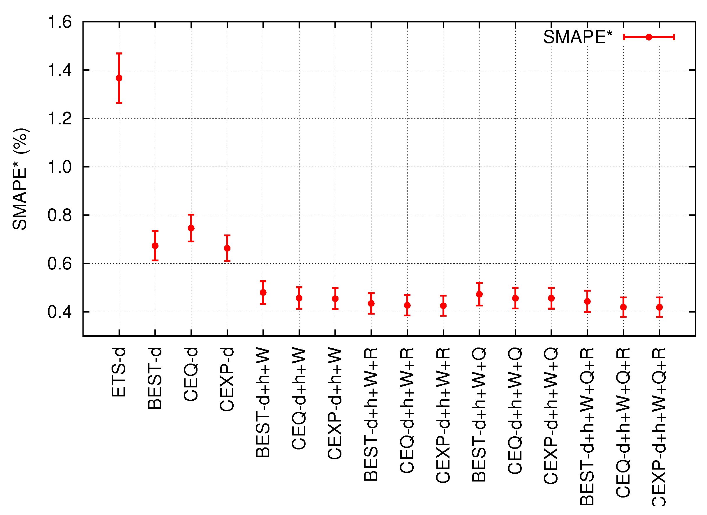
Finally, to compare the generalization abilities of the proposed best models, the error measures for the test partition are shown in Table 5 and Figure 7. All error measures show better performance in the test partition, even when this partition is two weeks ahead of training and contains hotter days than the training and validation partitions. The reason for this better performance might be that the test series has increasing/decreasing temperature cycles that are more similar to the training partition than the cycles in the validation partition. The differences between models are similar, and the most significant combination of covariates is time hour and sun irradiance ($d+h+W$) following the COMB-EXP strategy, achieving a SMAPE${}^{*}\approx 0.45\%$, MAE${}^{*}\approx 0.11$, and RMSE${}^{*}\approx 0.13$.

Table 5. SMAPE${}^{*}$, MAE${}^{*}$ and RMSE${}^{*}$ results on test partition comparing the best models with the $99\%$ confidence interval. Bolded face numbers are the best results, and the gray marked row is the most significant combination of covariates.

Model	SMAPE${}^{*}(\%)[lower,upper]$			MAE${}^{*}[lower,upper]$			RMSE${}^{*}[lower,upper]$
ETS-d	$1.3669$	$[1.2649,$	$1.4688]$	$0.3254$	$[0.3023,$	$0.3485]$	$0.3930$	$[0.3643,$	$0.4218]$
BEST-d	$0.6736$	$[0.6128,$	$0.7343]$	$0.1604$	$[0.1460,$	$0.1748]$	$0.2022$	$[0.1844,$	$0.2199]$
CEQ-d	$0.7462$	$[0.6907,$	$0.8016]$	$0.1767$	$[0.1638,$	$0.1895]$	$0.2203$	$[0.2046,$	$0.2360]$
CEXP-d	$0.6630$	$[0.6101,$	$0.7159]$	$0.1572$	$[0.1450,$	$0.1694]$	$0.1976$	$[0.1824,$	$0.2127]$
BEST-$d+h+W$	$0.4802$	$[0.4339,$	$0.5266]$	$0.1143$	$[0.1035,$	$0.1252]$	$0.1382$	$[0.1252,$	$0.1512]$
CEQ-$d+h+W$	$0.4569$	$[0.4127,$	$0.5012]$	$0.1090$	$[0.0985,$	$0.1195]$	$0.1318$	$[0.1193,$	$0.1443]$
CEXP-$d+h+W$	$0.4546$	$[0.4111,$	$0.4982]$	$0.1085$	$[0.0981,$	$0.1189]$	$0.1312$	$[0.1188,$	$0.1437]$
BEST-$d+h+W+R$	$0.4350$	$[0.3925,$	$0.4774]$	$0.1034$	$[0.0935,$	$0.1132]$	$0.1255$	$[0.1136,$	$0.1374]$
CEQ-$d+h+W+R$	$0.4271$	$[0.3854,$	$0.4688]$	$0.1013$	$[0.0916,$	$0.1111]$	$0.1225$	$[0.1109,$	$0.1341]$
CEXP-$d+h+W+R$	$0.4253$	$[0.3837,$	$0.4670]$	$0.1010$	$[0.0913,$	$0.1108]$	$0.1223$	$[0.1107,$	$0.1339]$
BEST-$d+h+W+Q$	$0.4727$	$[0.4258,$	$0.5196]$	$0.1127$	$[0.1015,$	$0.1238]$	$0.1353$	$[0.1223,$	$0.1483]$
CEQ-$d+h+W+Q$	$0.4565$	$[0.4136,$	$0.4994]$	$0.1092$	$[0.0988,$	$0.1195]$	$0.1314$	$[0.1192,$	$0.1436]$
CEXP-$d+h+W+Q$	$0.4565$	$[0.4134,$	$0.4995]$	$0.1091$	$[0.0988,$	$0.1195]$	$0.1313$	$[0.1192,$	$0.1435]$
BEST-$d+h+W+Q+R$	$0.4434$	$[0.3997,$	$0.4872]$	$0.1051$	$[0.0949,$	$0.1153]$	$0.1268$	$[0.1147,$	$0.1388]$
CEQ-$d+h+W+Q+R$	$0.4195$	$[0.3792,$	$0.4597]$	$0.0996$	$[0.0903,$	$0.1090]$	$0.1201$	$[0.1090,$	$0.1312]$
CEXP-$d+h+W+Q+R$	$\mathbf{0}.\mathbf{4192}$	$[0.3790,$	$0.4595]$	$\mathbf{0}.\mathbf{0994}$	$[0.0902,$	$0.1087]$	$\mathbf{0}.\mathbf{1200}$	$[0.1089,$	$0.1311]$

Table 5. SMAPE${}^{*}$, MAE${}^{*}$ and RMSE${}^{*}$ results on test partition comparing the best models with the $99\%$ confidence interval. Bolded face numbers are the best results, and the gray marked row is the most significant combination of covariates.

Model	SMAPE${}^{*}(\%)[lower,upper]$			MAE${}^{*}[lower,upper]$			RMSE${}^{*}[lower,upper]$
ETS-d	$1.3669$	$[1.2649,$	$1.4688]$	$0.3254$	$[0.3023,$	$0.3485]$	$0.3930$	$[0.3643,$	$0.4218]$
BEST-d	$0.6736$	$[0.6128,$	$0.7343]$	$0.1604$	$[0.1460,$	$0.1748]$	$0.2022$	$[0.1844,$	$0.2199]$
CEQ-d	$0.7462$	$[0.6907,$	$0.8016]$	$0.1767$	$[0.1638,$	$0.1895]$	$0.2203$	$[0.2046,$	$0.2360]$
CEXP-d	$0.6630$	$[0.6101,$	$0.7159]$	$0.1572$	$[0.1450,$	$0.1694]$	$0.1976$	$[0.1824,$	$0.2127]$
BEST-$d+h+W$	$0.4802$	$[0.4339,$	$0.5266]$	$0.1143$	$[0.1035,$	$0.1252]$	$0.1382$	$[0.1252,$	$0.1512]$
CEQ-$d+h+W$	$0.4569$	$[0.4127,$	$0.5012]$	$0.1090$	$[0.0985,$	$0.1195]$	$0.1318$	$[0.1193,$	$0.1443]$
CEXP-$d+h+W$	$0.4546$	$[0.4111,$	$0.4982]$	$0.1085$	$[0.0981,$	$0.1189]$	$0.1312$	$[0.1188,$	$0.1437]$
BEST-$d+h+W+R$	$0.4350$	$[0.3925,$	$0.4774]$	$0.1034$	$[0.0935,$	$0.1132]$	$0.1255$	$[0.1136,$	$0.1374]$
CEQ-$d+h+W+R$	$0.4271$	$[0.3854,$	$0.4688]$	$0.1013$	$[0.0916,$	$0.1111]$	$0.1225$	$[0.1109,$	$0.1341]$
CEXP-$d+h+W+R$	$0.4253$	$[0.3837,$	$0.4670]$	$0.1010$	$[0.0913,$	$0.1108]$	$0.1223$	$[0.1107,$	$0.1339]$
BEST-$d+h+W+Q$	$0.4727$	$[0.4258,$	$0.5196]$	$0.1127$	$[0.1015,$	$0.1238]$	$0.1353$	$[0.1223,$	$0.1483]$
CEQ-$d+h+W+Q$	$0.4565$	$[0.4136,$	$0.4994]$	$0.1092$	$[0.0988,$	$0.1195]$	$0.1314$	$[0.1192,$	$0.1436]$
CEXP-$d+h+W+Q$	$0.4565$	$[0.4134,$	$0.4995]$	$0.1091$	$[0.0988,$	$0.1195]$	$0.1313$	$[0.1192,$	$0.1435]$
BEST-$d+h+W+Q+R$	$0.4434$	$[0.3997,$	$0.4872]$	$0.1051$	$[0.0949,$	$0.1153]$	$0.1268$	$[0.1147,$	$0.1388]$
CEQ-$d+h+W+Q+R$	$0.4195$	$[0.3792,$	$0.4597]$	$0.0996$	$[0.0903,$	$0.1090]$	$0.1201$	$[0.1090,$	$0.1312]$
CEXP-$d+h+W+Q+R$	$\mathbf{0}.\mathbf{4192}$	$[0.3790,$	$0.4595]$	$\mathbf{0}.\mathbf{0994}$	$[0.0902,$	$0.1087]$	$\mathbf{0}.\mathbf{1200}$	$[0.1089,$	$0.1311]$

Figure 7. SMAPE${}^{*}$ error plot with the $99\%$ confidence interval for the models of Table 5 in the test partition.

Figure 7. SMAPE${}^{*}$ error plot with the $99\%$ confidence interval for the models of Table 5 in the test partition.

In order to perform a better evaluation, the conclusions above are compared with mutual information (MI), shown in Table 6. Probability densities have been estimated with histograms, making the assumption of independence between time points, which is not true for time series [39], but is enough for our contrasting purpose. The behavior of the ANNs is similar to the MI study. Sun irradiance (W) covariates show high MI with indoor temperature (d), which is consistent with our results. Humidity (H) and air quality (Q) MI with indoor temperature (d) is higher than sun irradiance, which seems contradictory with our expectations. However, if we compute MI only during the day (removing the night data points), the sun irradiance shows higher MI with indoor temperature than other covariates. Regarding the hour covariate, it shows lower MI than expected, probably due to the cyclical shape of the hour, which breaks abruptly with the jump between 23 and 0, affecting the computation of histograms.

Table 6. Mutual Information (MI) and normalized MI between considered covariates and the indoor temperature, for the validation set.

Data	Algorithm	d	h	W	H	R	Q
	MI (for d)	$9.24$	$4.44$	$6.06$	$8.95$	$0.51$	$7.70$
Validation set	Normalized MI (for d)	$2.00$	$1.48$	$1.65$	$1.95$	$1.06$	$1.82$
Validation set,	MI (for d)	$8.23$	$3.50$	$8.11$	$8.09$	$0.58$	$7.41$
removing night data points	Normalized MI (for d)	$2.00$	$1.42$	$1.98$	$1.97$	$1.07$	$1.89$

Table 6. Mutual Information (MI) and normalized MI between considered covariates and the indoor temperature, for the validation set.

Data	Algorithm	d	h	W	H	R	Q
	MI (for d)	$9.24$	$4.44$	$6.06$	$8.95$	$0.51$	$7.70$
Validation set	Normalized MI (for d)	$2.00$	$1.48$	$1.65$	$1.95$	$1.06$	$1.82$
Validation set,	MI (for d)	$8.23$	$3.50$	$8.11$	$8.09$	$0.58$	$7.41$
removing night data points	Normalized MI (for d)	$2.00$	$1.42$	$1.98$	$1.97$	$1.07$	$1.89$

6. Conclusions

An overview of the monitoring and sensing system developed for the SMLsystem solar powered house has been described. This system was employed during the participation at the Solar Decathlon Europe 2012 competition. The research in this paper has been focused on how to predict the indoor temperature of a house, as this is directly related to HVAC system consumption. HVAC systems represent $53.89\%$ of the overall power consumption of the SMLsystem house. Furthermore, performing a preliminary exploration of the SMLsystem competition data, the energy used to maintain temperature was found to be $30\%$–$38.9\%$ of the energy needed to lower it. Therefore, an accurate forecasting of indoor temperature could yield an energy-efficient control.

An analysis of time series forecasting methods for prediction of indoor temperature has been performed. A multivariate approach was followed, showing encouraging results by using ANN models. Several combinations of covariates, forecasting model combinations, comparison with standard statistical methods and a study of covariate MI has been performed. Significant improvements were found by combining indoor temperature with the hour categorical variable and sun irradiance, achieving a MAE${}^{*}\approx 0.11$ degrees Celsius (SMAPE${}^{*}\approx 0.45\%$). The addition of more covariates different from hour and sun irradiance slightly improves the results. The MI study shows that humidity and air quality share important information with indoor temperature, but probably, the addition of these covariates does not add different information from which is indicated by hour and sun irradiance. The combination of ANN models following the softmax approach (COMB-EXP) produce consistently better forecasts, but the differences are not important. The data available for this study was restricted to one month and a week of a Southern Europe house. It might be interesting to perform experiments using several months of data in other houses, as weather conditions may vary among seasons and locations.

As future work, different techniques for the combination of forecasting models could be performed. A deeper MI study to understand the relationship between covariates better would also be interesting. The use of second order methods to train the ANN needs to be studied. In this work, for the ANN models, the hour covariate is encoded using 24 neurons; other encoding methods will be studied, for example, using splines, sinusoidal functions or a neuron with values between 0 and 23.

Following these results, it is intended to design a predictive control based on the data acquired from ANNs, for example, from this one that is devoted to calculating the indoor temperature, extrapolating this methodology to other energy subsystems that can be found in a home.