1. Introduction
Mobile mapping system (MMS) is a photogrammetric mapping agent that is usually defined as a set of navigation (global navigation satellite system (GNSS) and inertial measurement unit (IMU)) and remote sensors—such as cameras, lidar, and odometer sensors—integrated in a common moving platform [
1]. The importance of an MMS has been widely highlighted based on its cost-effectiveness, high data-capturing rate, and acceptable level of accuracy [
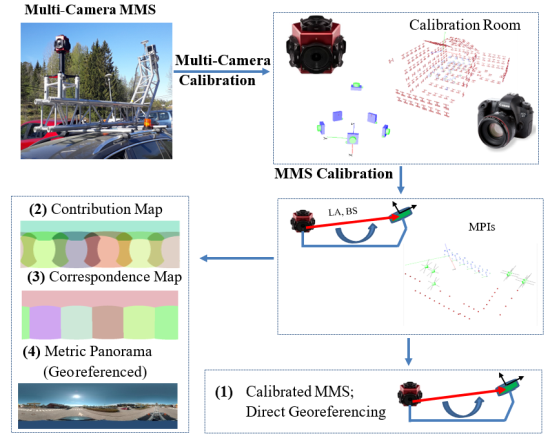
2]. System calibration is an indispensable part of the process of employing an MMS. Regarding an MMS that is based on multi-cameras and navigational systems, two calibration process could be mentioned: multi-camera calibration and MMS calibration. Multi-camera calibration aims to estimate interior and relative orientations of a multi-camera. MMS calibrations refers to estimating relative position and orientation between a multi-camera and GNSS/IMU sensors. Accurate system calibration ensures high-quality outputs for at-least a minimum period that a mapping system stays relatively still; a periodic system calibration scheme is able to guarantee the correctness of time-dependent parameters.
The first aspect of employing an optical-based MMS relates to the problem of multi-camera calibration [
2,
3,
4,
5,
6,
7,
8,
9,
10,
11]. Nowadays, many MMSs are equipped with multi-projective cameras (MPC) because of their sturdy design, large field of view (FOV), and promising sensor models. Sensor modeling of an MPC usually consists of interior orientation parameters (IOP) of individual cameras, relative orientation parameters (ROP) between cameras with respect to a reference camera, and a scale factor that connects ROPs to a global framework. An important aspect of integrating a camera system in an MMS relates to the problem of employing a rigorous sensor model that fits to the physics of the camera. The sensor model maps a 3D object point into its corresponding image point [
12]. The next step is to employ the sensor model as the core of a statistical optimization model to find optimum values and express our uncertainties about the unknowns such as camera parameters or 3D position of object points.
Many MMSs use multiple cameras but do not necessarily generate panoramas. A panorama is a continuous presentation of an environment which is demonstrated by one photo or a series of photos that are merged together by a ‘stitching’ or a ‘geometric non-stitching’ approach. This form of photography provides viewers with an unlimited viewing possibility in all directions [
12]. Because of the all-angle viewing property, panoramic photography has found a wide range of applications; few of those applications are computer vision, robotics, surveillance, virtual reality, indoor/outdoor photography, and historical heritage documentation.
Recently developed photogrammetric models for MPCs has brought a new perspective in panoramic images applications. If these cameras, which are initially designed for all-direction photography, treated with photogrammetric models, numerous potential applications will emerge for surveying and mapping purposes.
A categorization of panoramic cameras can help us to find shared properties and mathematical model for members of each class. Amiri Parian and Gruen [
12] categorized panoramic imaging into four groups: stitched, mirror-based rotating-head, near 180, and scanning 360 panoramas. Stitched panoramas are mainly used for non-metric applications where accurate directions are not important; therefore, this class is outside the focus of a metric categorization. We may re-categorize most of commercially available panoramic cameras that are suitable for surveying tasks according to their internal capturing technology into four groups [
13]: (1) rotating-head, (2) multi-fisheye and (3) multi-projective camera, and (4) catadioptric systems. The benefits of the latter categorization are twofold. Most of commercially available cameras that are useful in metric photogrammetry tasks fit into this categorization; moreover, it simplifies the sensor modeling since it has founded based on a similarity measure that places cameras to a category according to their common sensor model.
The category (1) rotating head cameras contains cameras based on linear array CCDs that is mounted on a vertically rotating head. Examples of this class include EYESCAN M3 that is jointly developed by DLR and KST [
14] and SpheroCam which is manufactured by SpheronVR AG. Equivalently, a projective camera such as a Canon EOS 6D could be mounted on a motorized rotating head such as Phototechnik AG, Roundshot metric, piXplorer 500, or GigaPan EPIC pro. The camera and step motors are synchronously controlled by a central processing Unit (CPU) that plans the movements and takes image shots. If the system has been accurately calibrated (optical center of the projective camera’s lens should be precisely located on the center of rotation), high-precision metric information and high-resolution panoramic images can be obtained with least effort [
15]. Depending on the target applications, one or two step motors are working simultaneously to rotate the central camera around a point/axe. One main configurable parameter in building this class is the option to choose between one or two rotating axes; a post-processing module is responsible to transfer and merge images that have been captured with different orientations. Subsequently, a color blending approach is required to ensure that color tunes between stitched images are consistent. Usually a full resolution shot takes few seconds to even few minutes to compile which makes this class of panoramic cameras relatively unsuitable for mobile-mapping. Some important use-case of this class is cultural heritage recording and classification [
16,
17], high-precision surveying [
12,
18,
19,
20,
21], industrial-level visualization, indoor visualization, 3D modeling, and artistic photography.
The category (2) multi-fisheye cameras comprises a structure of a dual spherical camera module mounted on a rigid frame to construct a light-weight mobile 360 imaging system; Few consumer-grade samples of this class are Samsung Gear 360 [
22], SVPro VR 360, MoFast 720, MGCOOL cam 360, SP6000 720, Ricoh Theta S [
7]. Some recent works suggests multi-camera system based on a dual-fisheye design [
23,
24]. Fisheye camera models for photogrammetric applications were extensively studied and tested [
25,
26,
27,
28,
29]. The simultaneous geometric calibration of multi-camera system based on fisheye images, aiming a 360° field of view also started to be discussed recently. For instance, a dual fisheye calibration model is proposed by [
30] and [
7]. For this class of cameras, a customized statistical optimization process that involves using weighted observations and initial distributions of unknowns has proved sufficiently accurate for low to medium-accuracy surveying applications. However, some limitation of these systems can be mentioned, such as non-perspective inner geometry, huge scale and illumination variations between scenes, large radial distortion and nonuniformity of spatial resolution. Therefore, the overall image quality of panoramic images that are produced by the cameras of this class are usually worse than the first or third categories, however, some desired aspects—such as data-capturing rate or simplicity—makes them ideal candidates for applications such as low accuracy mobile mapping or 3D virtualization [
31,
32,
33,
34,
35].
The category (3) multi-projective cameras contains panoramic cameras with arbitrary number of projective cameras mounted fix on a rigid frame (an industrial examples is LadyBug with six cameras [v.3 and v.5;
] by FLIR; a consumer-grade example is Panono 360 with 36 cameras [
]). Cameras of this class (multi-projective cameras or in short MPC) are usually customized for certain imaging, navigation, or surveying tasks. A synchronous shutter mechanism is applied to take simultaneous shots (<1 msec delay). A geometric model for MPC integrated into a statistical adjustment model is proposed by many researchers, e.g., ([
9,
10,
11]). This model ensures desirable geometric accuracies for many tasks such as 3D mapping and surveying, 3D visualization, and texturing. Panoramas that are initially generated for this class are based on stitching techniques that mainly have visualization and artistic values; it is in contrast to the geometric values of panoramic images that are taken from cameras of the first or the second categories; this class of cameras has rigorously found many applications such as surveying, robotics, visualization, cinema, and artistic photography. Similar to the second class, it has the potential to be employed in applications that needs fast data-capturing rates such as mobile mapping, or navigation.
Early attempts to employ relative orientation constraints among multiple cameras was applied to a stereo camera, e.g., ([
3,
36,
37]). He et al. [
36] developed an MMS with a stereo camera and a GPS receiver to measure global coordinates of any point through photogrammetric intersection. King [
3] modified the conventional bundle block adjustment (BBA) to accept relative orientation stability constraints. Zhuang [
37] employed a fixed-length moving target to calibrate a stereo camera. Later, more complex systems of cameras went under research investigations. For example, Svoboda et al. [
38] calibrated an
that were installed on a visual room. Lerma et al. [
39] calibrated a
that consisted of a stereo camera and a thermal camera by employing distance constraints. Habib et al. [
40] analyzed variations in IOP/Exterior Orientation Parameter (EOP) of multi-cameras. Detchev et al. [
41] presented a system calibration scheme by employing system stability analysis. Some researchers employed a calibration field for multi-camera calibration. For example, Tommaselli et al. [
5] employed AURUCO coded targets [
42] to design a terrestrial calibration field. They used their proposed photogrammetric field to calibrate fisheye, catadioptric, and multi-cameras. Khoramshahi and Hokovaara [
10] employed a customized coded target (CT) to create a calibration room. They employed it to calibrate a complex
(Panono), and an
(LadyBug v.3). In this work, we follow the calibration model that was proposed by Khoramshahi and Honkavaara [
10].
Category (4) contains catadioptric systems that employ complex optical systems. A set of spherical and aspherical lenses, shaped mirrors such as parabolic, hyperbolic, or elliptical mirror [
43], and refractors are employed in catadioptric systems to cover a large FOV. An example of this class was proposed by [
23] as a prototype dual catadioptric camera. A calibration model for a catadioptric camera consists of a wide-lens camera and a conic mirror was proposed by [
44].
The second aspect of employing an MMS relates to the problem of direct geo-referencing. Using multi cameras of third category for mapping applications require accurate determination of orientation and position of each panorama. This orientation can be done by indirect or direct georeferencing techniques, or combining both. Direct geo-referencing is a very useful approach for real-time application such as mobile mapping, or aerial surveying. Direct geo-referencing is the process to find position and orientation of captured images (EOPs) in a global reference frame without employing any ground control point (GCP), which requires the integration of additional sensors such as GNSS receivers and IMU sensors into the camera’s mounted frame. This integration either provides initial values for positions and orientations of the camera shots as weighted observations in the BBA, or helps the system to instantly estimate position vectors and Euler angles of shots [
45]. It is worth noting that a successful direct geo-referencing requires two main aspects. Firstly, GNSS and IMU sensors should be accurately synchronized to an MPC. Secondly, a robust estimation of lever-arm vector and boresight angles should be known. These later parameters are known as mounting parameters [
46]. Rough estimation of the MMS calibration parameters could be performed by comparing observations of GNSS and IMU with the output of BBA. To enable a direct geo-referencing, a customized sensor model is required to be employed by considering additional parameters of lever-arm and boresight misalignments of an MPC with respect to GNSS and IMU sensors.
A variety of calibration schemes has been overly discussed in the literature; however, as far as the authors concerned, a rigorous, practical, and easy solution for direct georeferencing of an MPC does not exist that completely fit to the configuration of a multi-camera MMS. Moreover, stitching operation is required to compile a panorama from images of the third category cameras. This panoramic presentation usually has just artistic or visual values. A non-stitching panoramic creation scheme is also feasible for this class that adds geometric value to generated panoramas. This paper contributes to a rigorous, easy, and practical scheme for calibrating a multi-camera MMS equipped with an MPC, GNSS and IMU sensors in a terrestrial vehicle. We also present a novel non-stitching algorithm by introducing a panoramic correspondence map. We propose a modified BBA that comprises MPC calibration and MMS calibration. We assess quantitatively the quality of the proposed approach by checking the accuracy of the point intersection by independent checkpoints. Our results demonstrate that sub-decimeter level accuracy is achievable by this technique.
2. System Calibration
Mathematical theory behind the implementation of this work is discussed in this part. We first start with sensor model of an MPC, then we continue toward discussing a complete sensor model for the underlying MMS. Finally, a modified BBA is discussed to employ the sensor model and statistically express uncertainties about parameters.
2.1. Individual Camera Model
The following interior orientation model removes main distortions from image coordinates and outputs undistorted pinhole image coordinates as
where
and
are distorted coordinates of a point in pixel unit,
and
are coordinates of the principal point,
are radial distortion coefficients,
are tangential distortion parameters, and
and
are scale and shear factor respectively. It is trivial to show that the underlying model (Equation (1)) is exchangeable to Brown’s model [
47,
48].
An image of a projective camera is linked to the camera’s sensor model, and relates to six orientation and position parameters that uniquely determines it inside a 3D Euclidean space. Therefore, a linear relationship between an object point and its undistorted pinhole coordinates is established by the collinearity model
where
is the i
th row of the rotation matrix
,
is a vector of (3 × 1) of the object point’s coordinates, and
is a (3 × 1) vector of location of image in a 3D cartesian space (bold letters are used for vectors and matrices and normal letters are used for scalers throughout this paper).
2.2. Multi-Projective Camera Model
An MPC is presented in this work by the following calibration parameters:
() (),
(),()},
,
where is interior orientation parameters of an individual camera of an MPC, is relative orientation of an individual camera with respect to the first camera, are Euler angles, are displacements, and is the unknown scale factor. The last parameter () plays a role if scale of an MPC sensor would be different from scale of the model. It could be ignored if both scales are equal. In overall, there will be a number of calibration parameters for an MPC with (n) projective camera; a multi projective image (MPI) is geometrically defines by its corresponding MPC sensor and six EOPs.
2.3. Space Resection of Multi-Projective Images
The goal of the space resection is to find approximate locations of a given MPI with respect to a 3D frame under the conditions that at-least (3) image-object correspondences exist and localized in a 3D Cartesian framework. Space resection helps to orient a set of MPIs with respect to a given point set (e.g., a calibration room). The orientations are finally adjusted through a BBA.
An alternative way to resect an MPI is to employ the coplanarity equation. Coplanarity condition connects two normalized pinhole coordinates and image centers through a matrix called Essential, which is a (3 × 3) matrix that is composed of three rotations and three translations as
where
is the matrix presentation of a cross product which is a
matrix of the form
Essential matrix is estimated by the following equations
where
is normal image point at time (
), and
is the calculated normal location of the same 3D point in a synthesized image. Space resection of an MPI is performed for each of its projective images. At least 5–8 tie points are required based on the selected method (5-point [
49], 6-point, 8-point, or normalized 8-point [
50]). Then a synthesized pair is formed. The synthesized image is localized such that the resulted stereo pair becomes stable. Next, the retrieved position is translated into approximate position of the parent MPI (
); finally, all positions are averaged to estimate the position and orientation of the MPI
2.4. Relative Orientation between Two Multi-Projective Images
Finding ROPs between two MPIs is essential to independently construct a scene. ROPs between two MPIs are expressed by six parameters out of which five are independent. Usually the largest element of a stereo pair’s baseline is scaled to one. Three rotations and two displacements are finally solved by relative orientation module. To estimate ROPs between two MPIs, a similar averaging approach to the space resection has been chosen. Therefore, all image pairs between MPIs are oriented. Then the resultant ROPs are transformed to the parent MPI and averaged.
In the process of MMS calibration, initial values of lever-arm and boresight misalignments are estimated by independently compiling a local network of few shots, then connecting the local network to the global frame of GNSS/IMU sensors.
2.5. Bundle Block Adjustment
BBA employs non-linear least-square adjustment method to minimize a cost function based on residuals of observational equations. It finally expresses the uncertainties about the unknowns of an MPC calibration as a covariance matrix. The MPC cost function is a combination of all observational equations. It is expressed as the vector function
where,
are IOPs for projective cameras (1:n),
are structural parameters regarding the
,
are orientations and locations of image shots,
are position of object points and the corresponding image points,
and
are lever-arm vector and boresight misalignments respectively. To model the entire system, equations for image observations, GNSS/IMU-observations, and GCPs are introduced.
Two observational equations are considered in the MPC’s BBA for each image tie points, as
In Equations (8) and (9),
are pinhole coordinates of object point (
) inside image (
) (pinhole camera, f = 1),
is the (
) row of the rotation matrix
(
projective camera [
] at time
),
is location of
projective camera at time
, and
is 3D location of the corresponding object point (
).
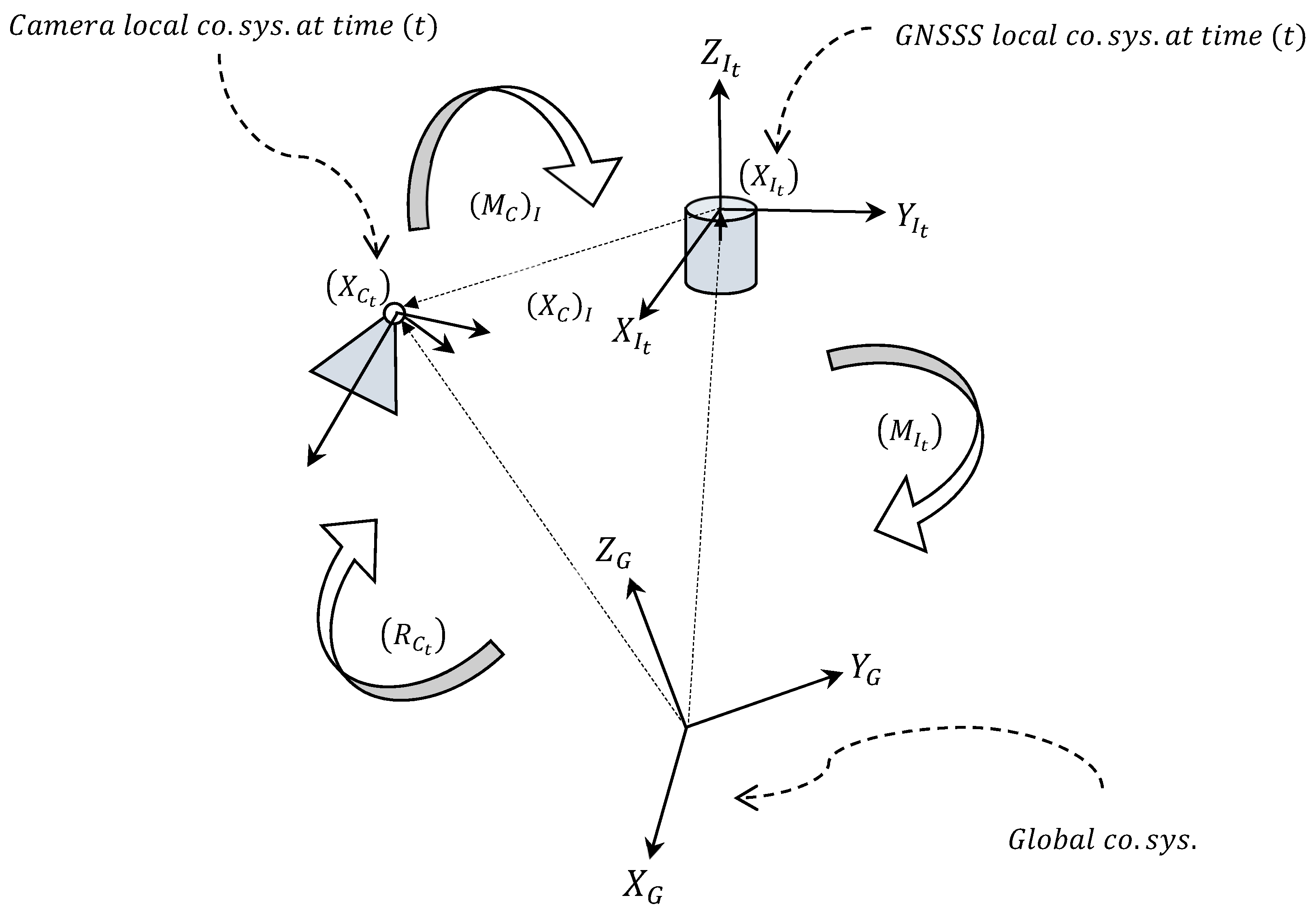
In order to combine observations of GNSS and IMU sensors to the BBA, a link between GNSS, IMU and the MPC is established (
Figure 1). A number of (6) additional parameters are introduced to represent a shift (lever-arm), and orientations (boresight misalignments). The connection is formulated by six non-linear equations (Equations (10) and (11)). The observational equation for lever- arm and boresight misalignments are
where
are ‘observed’ Euler angles of the INS at time (
),
is the rotation matrix of an MPC with respect to the INS local coordinate system, and
is rotation matrix of the MPC at time (
). In Equation (11),
is observed position of INS at time (
),
is unknown position of the MPC at time (
), and
is relative position of the camera with respect to the INS in the local coordinate system of the INS. Here,
indicates the function that maps a rotation matrix into its corresponding Euler angles.
GCPs are contributed to the BBA by three observational equations
where
is unknown 3D position of a GCP, and
is observed position.
2.6. Panoramic Compilation
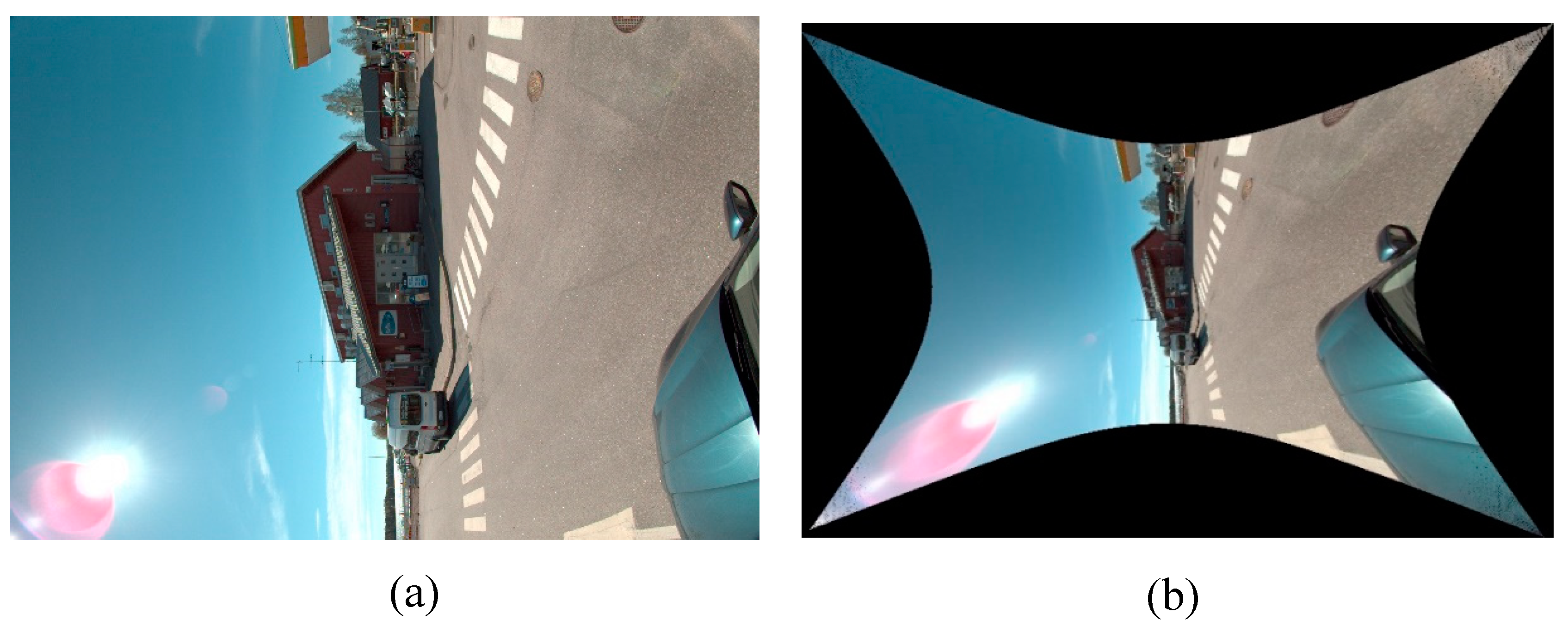
Creating a panorama for an MPC without image stitching is possible under the condition that the MPC is calibrated (known IOPs and ROPs). Therefore, calibration data is sufficient to compile a non-stitching panorama. The algorithm for building a panorama contains looping over a hypothetical sphere or cylinder (optional projection system) that covers an MPI, then for each pixel in the final panoramic compilation the algorithm finds a corresponding camera index (0-n) and an image location (pix). For a better rendering result, an appropriate interpolation technique (bilinear or bicubic) could be considered since the projection from the sphere (or cylinder) to projective images results in subpixel positions. If the correspondence data is saved as a meta-data file (it may be called panoramic correspondence map), then the final panorama will have geometric values. It is because of the fact that collinearity condition between an object point, its corresponding image point, and perspective center of a projective camera of an MPC is established. A second usage of the correspondence map is efficiently compiling a panorama, since indexing is expected to be much quicker than direct calculation.
There are regions in the correspondence map that more than one choice of correct image is possible for every point in the final panoramic compilation. It is because of the existence of overlaps between adjacent cameras. A criterion needs to be considered to build a unique map, for example minimum incident angle could be used.
Depending on the distance of a 3D object points to a panorama, discontinuity on edges is expected to occur; it is because the projection center of different individual cameras does not match to the center of the hypothetical sphere. Discontinuity is expected to be more severe for closer objects. Finally, an important post-processing is the use of color blending on edges. It improves the quality of a compiled panorama. Without color blending, sharp steps are expected to be observed on the edges that pixel labels start to switch from one camera to another. Color blending softens those steps and improves the color consistency of the final panorama.
3. Methods and Material
3.1. Mobile Mapping System
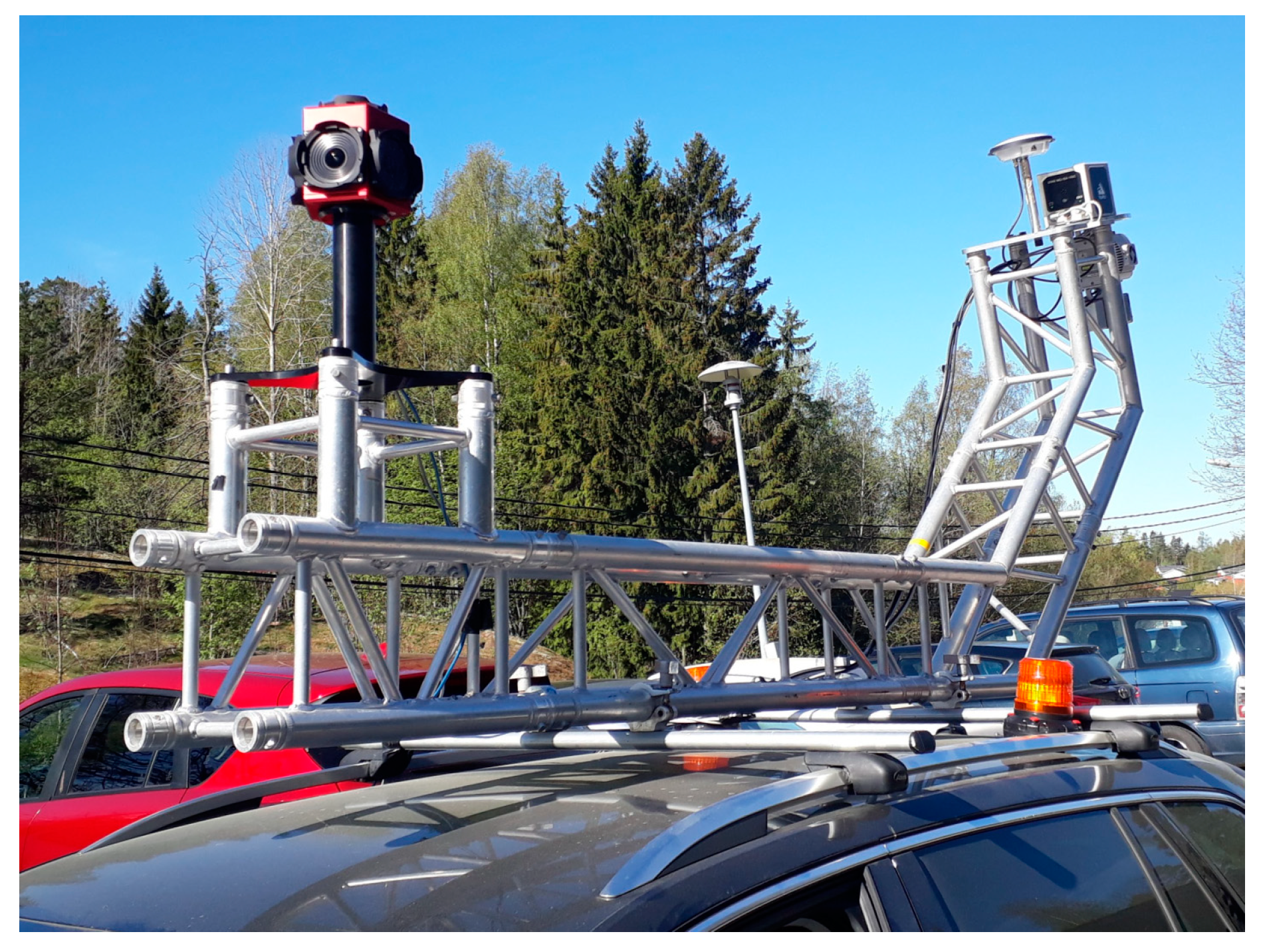
The MMS in this works comprises an MPC, a GNSS, and an IMU that are firmly installed on a car’s roof. This section describes the experiments to assess the proposed method described in
Section 2. The proposed method was implemented in C++ and MATLAB languages and evaluated using a real dataset from an MMS composed by a multi-camera LadyBug 5, and a navigation system installed on a rigid aluminum truss structure on top of a Skoda Superb (
Figure 2).
Ladybug V.5 is an MPC with five side-looking cameras and one upward-looking camera. Each individual camera contains a sensor of size 2464 × 2048 pix. Its focal length is 18 mm with sensor size of (35.8 × 29.7 mm) with field of view of . Panoramas cover an area of 360 horizontally by 145 vertically. Resolution of output panoramas is approximately 8k (7200 × 3600 pixels, aspect ratio 2:1).
The GNSS receiver used was a NovAtel PwrPak7, which together with IMU compiles a Synchronized Position Attitude Navigation (SPAN) system. PwrPak7 logged GPS and Glonass observations via NovAtel VEXXIS GNSS-850 satellite antenna. Sensor trajectory was computed by combining GNSS and IMU data with Waypoint Inertial Explorer software. Virtual GNSS base station reference data was acquired from commercial Trimnet service. The maximum distance from trajectory (
Figure 3) to the base station was ~350 meters. The 3D RMSE for the GPS positions was 1.6 centimeters.
A NovAtel IMU-ISA-100C, manufactured by Northrop-Grumman Litef GMBH, was paired with a NovAtel SPAN GNSS receiver. The IMU-ISA-100C is a near navigation grade sensor containing GNSS-850 satellite antenna (in front of IMU) mounted on a truss structure on top of a Skoda passenger car. NovAtel PwrPak7 GNSS receiver together with operating and logging laptop were inside the car.
3.2. MPC Calibration
FGI’s calibration room is an empty space with dimension of 519 × 189 × 356 cm
3 that is equipped with 215 CTs (
Figure 4). 3D positions of all targets are a-priori known based on previous observations. Images taken with a Canon EOS 6D camera (sensor 20 Megapixel, image size 5472 × 3648
, lens Canon EF 24 mm, focal length
) were used to accurately calculate 3D coordinates of the targets [
10] in the calibration room with bundle adjustment, before MPC calibration.
In the first step, FGI’s camera-calibration room was employed to calibrate the MPC. To do so, 3D positions of the CTs had been accurately estimated by employing a Canon EOS-6D camera achieving a relative 3D positioning precision of std < 1 mm. The automatic target extraction included:
Employing adaptive thresholding using first-order statistics to roughly estimate the position of blobs (accuracy of better than 2pixel);
Accurately fitting rotated ellipses to extracted blobs by least-square fitting (accuracy 0.1 pixel),
Clustering blobs;
Finding CTs from extracted clusters by employing structural signature of the CTs, and
Reading ID for each target.
The automatic CT detection was implemented in MATLAB. The standard deviation for image-point observations was set as 0.1 pixel.
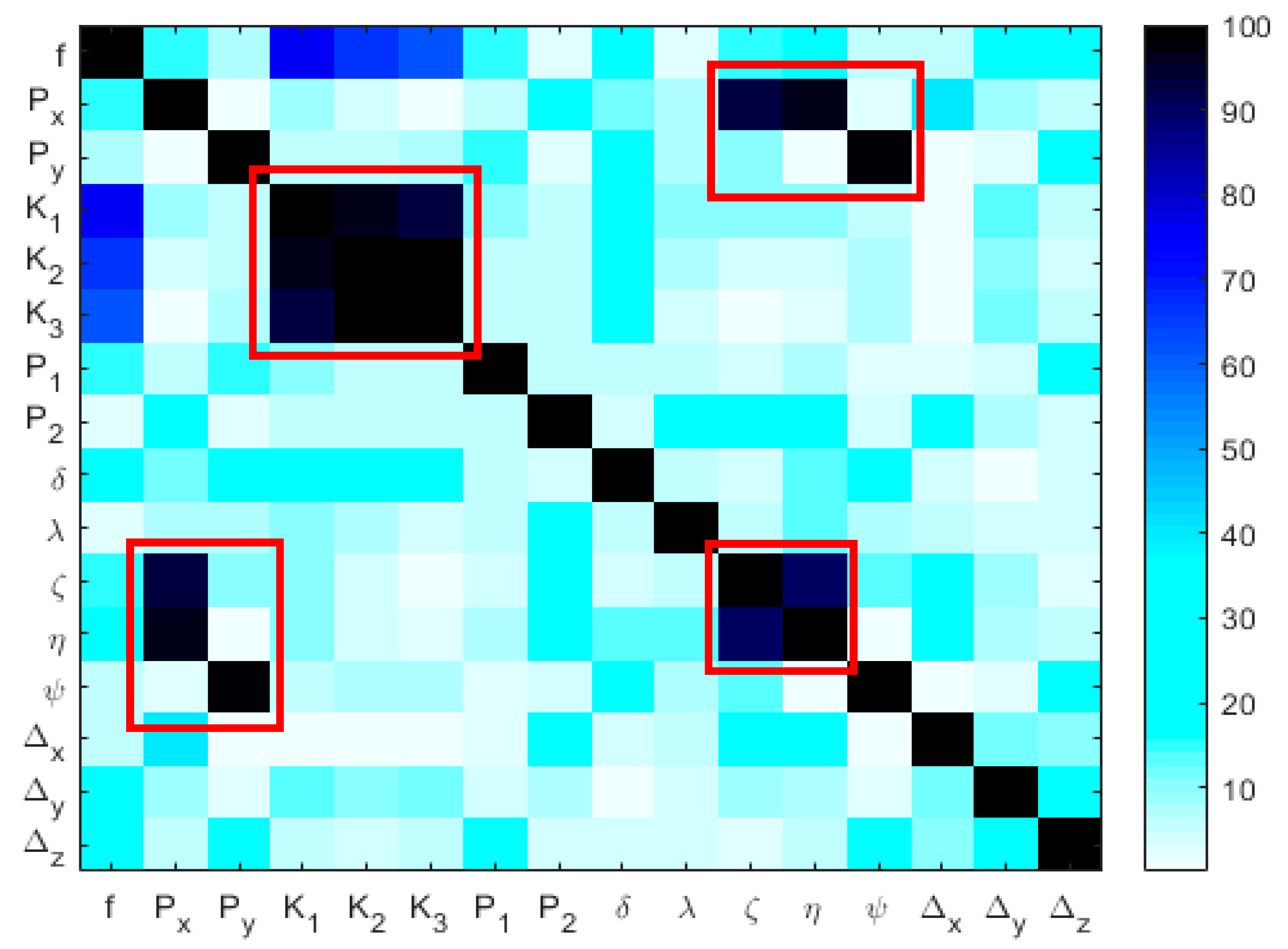
The estimated focal length of the Canon was 3156.10 pixels with a standard deviation of 0.04 pixels. The principal point was estimated as (2752.37, 1509.36) pixels with standard deviation of 0.05 pixels. Regarding each of the IOPs, a significance analysis is performed assessing the amount of distortion that is corrected by freezing all the IOPs except for an underlying parameter (or set of parameters) on a grid of 10 × 10 pixels. The largest distortion on the grid was chosen as significance value for a given IOP. The significance values for radial distortions (set), tangential distortion (P1, P2, and P3), scale, and shear were 69.2, 2.4, 1.0, 0.03, and 0.06 pixel respectively. The estimated standard deviations of the CT points were 0.15, 0.03, and 0.02 mm in principal directions of 3D error ellipsoids respectively, which indicates that our target accuracy was achieved.
In the second step, the same CTs were automatically extracted in individual images of the MPC (LadyBug 5). Next, each MPI was resected (
Section 2.3) using the calibration-room’s CTs, and finally, the BBA was performed to optimize the sensor parameters of the MPC. In this processing, the CTs coordinates based on the measurement by the Canon were kept fixed.
Two datasets of 26 and 53 MPIs were captured from the FGI’s calibration room to calibrate the MPC. In the first dataset, the camera is attached to a horizontal slide, therefore each few images are coplanar and at the same height level. In the second dataset, the camera is put on a tripod with two different height levels. In total, 474 individual projective images have been captured; then, CTs were automatically extracted in all individual images.
3.3. MMS Calibration
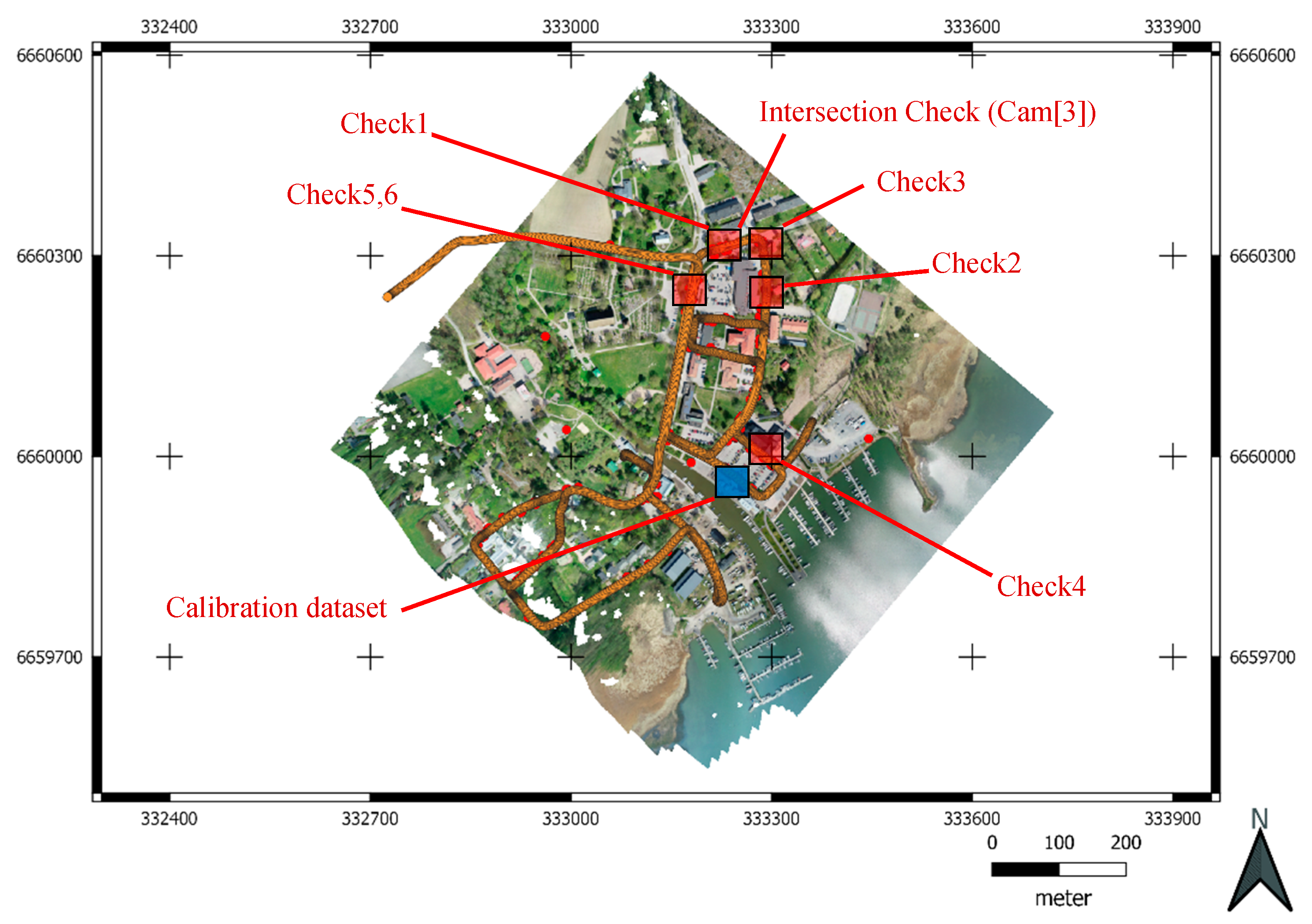
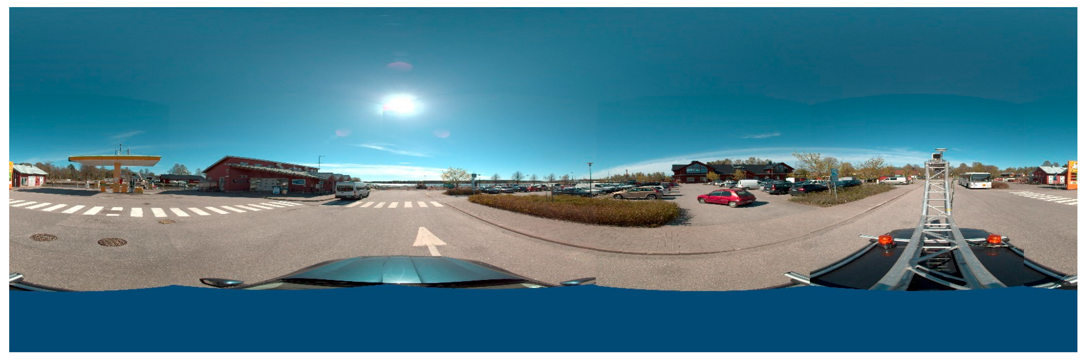
The MMS calibration was carried out using outdoor dataset from Inkoo, which is a municipality in southern Finland. A set of 8424 MPIs were captured by the LadyBug 5 camera for Inkoo harbour area and two close-by regions. Most roads have been captured by the MMS in both directions.
The GCPs were measured using the Topcon Hiper HR RTK dual band receiver with an accuracy within 5 mm + 0.5 ppm horizontally and 10 mm + 0.8 ppm vertically [1. source:TOPCON]. Nearest base station was located in Metsähovi 28 km away from Inkoo, therefore accuracy is vertically 19.0 mm and horizontally 32.4 mm, respectively.
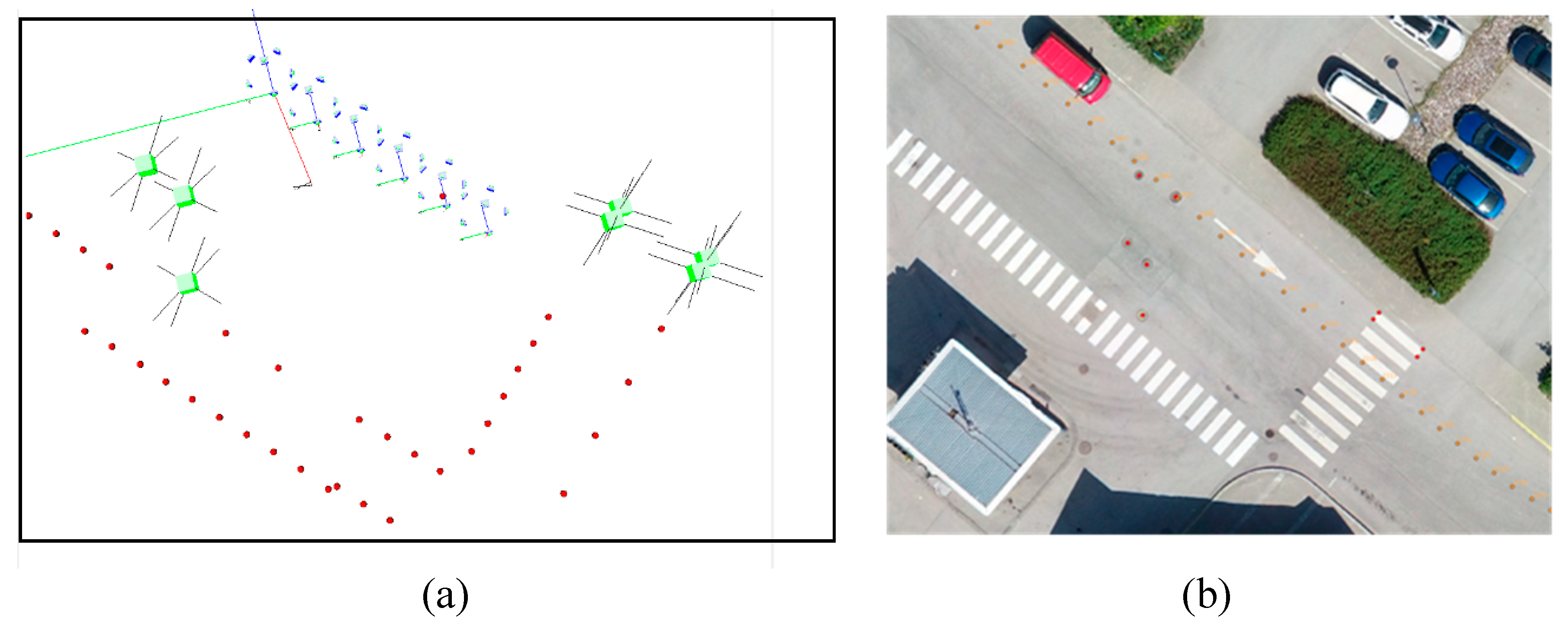
The MMS calibration involved estimating relative parameters of the MPC with respect to the GNSS and IMU (lever-arm and boresight miss-alignments). Observational Equations (10) and (11) were added to BBA. Analytical partial derivatives of latter equations were considered for calculating the Jacobian matrix. The calibrated MPC sensor was used to construct an outdoor case. The sensor was kept fixed during the scene reconstruction except for its scale parameter. A number of six MPIs were connected together by the relative orientation module (
Section 2.4) to construct a local network (initial network). Model coordinates of all 3D points were accurately determined with corresponding sub-pixel re-projection error and added as observational equations. Few GCPs were observed in individual images and added to the model to establish a link to the global coordinate system (Equation (6)). Then, GNSS and IMU observations were added to the initial network. Lever-arm and boresight was initialized from the initial network and finally optimized through the BBA. The MPC sensor kept fixed during MMS calibration to avoid a singularity in the Jacobian matrix. In the optimization process, locations, and orientations of MPIs, 3D positions of GCPs, and six parameters of lever-arm and boresight were set free.
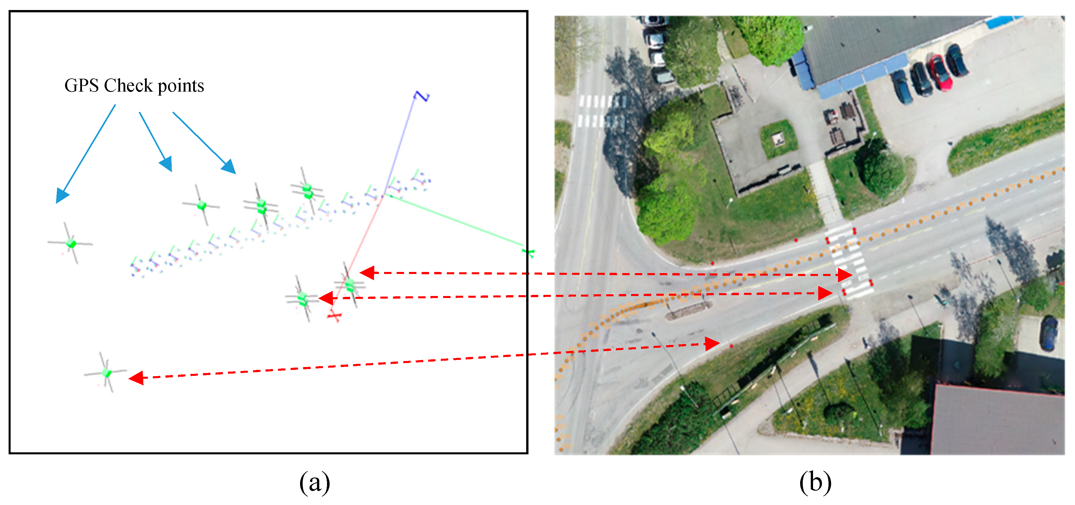
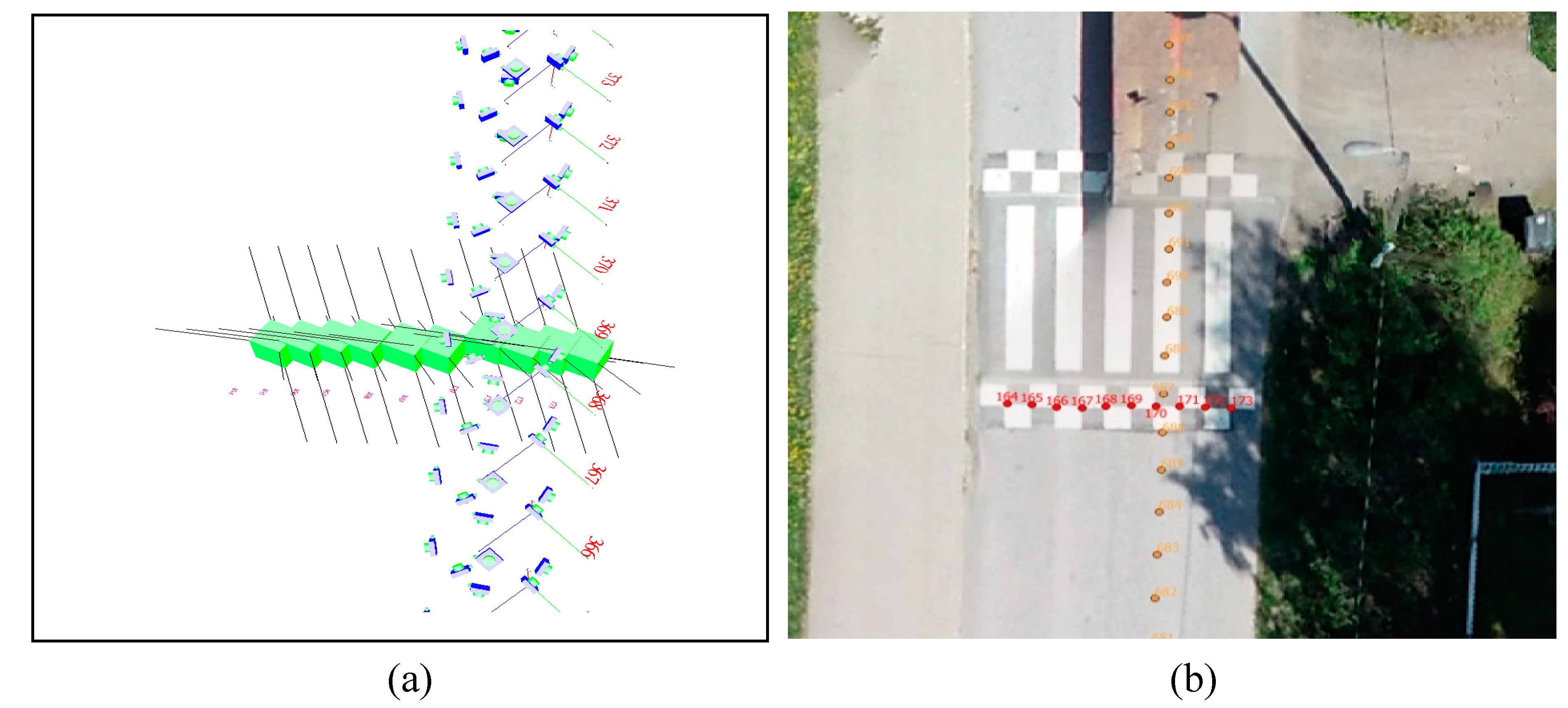
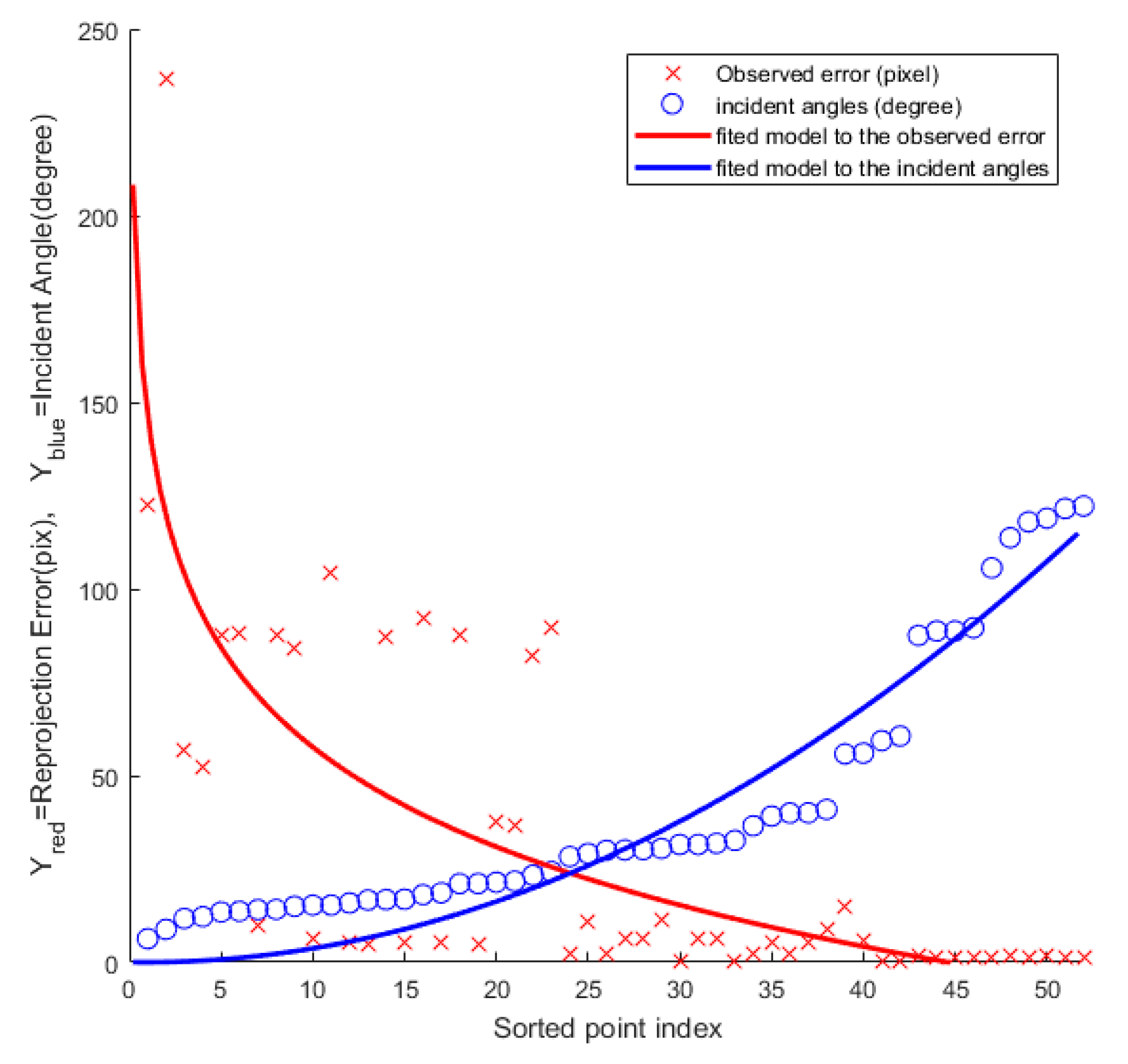
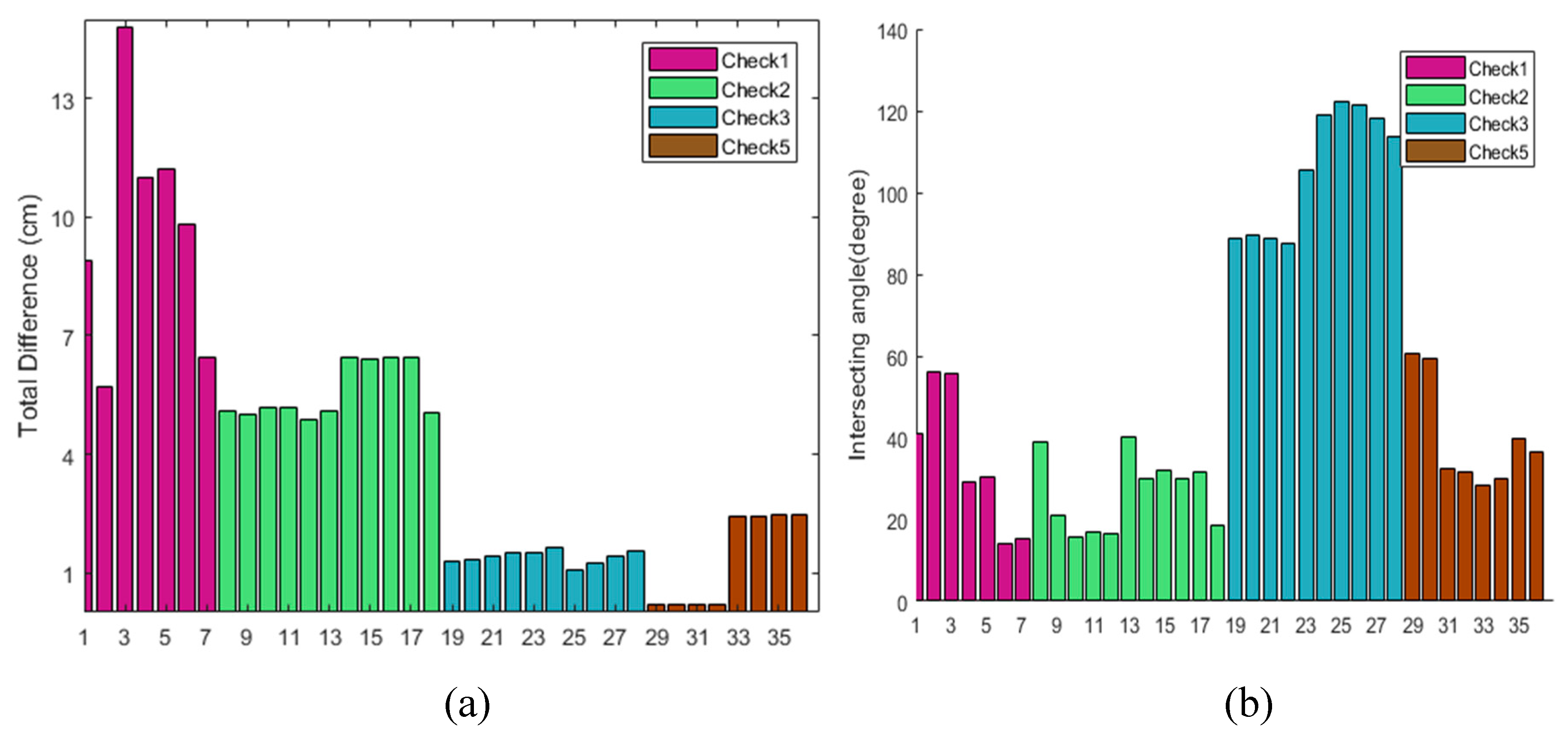
3.4. Performance Assessment
In order to assess the accuracy of the MMS calibration and georeferencing, seven check sites approximately covering the area were selected (
Figure 3). In each site, the GNSS and IMU readings of the MMS were translated into MPI orientations that were converted into individual image’s orientation and rotation by using MPC sensor calibration information from Step 1 (
Section 3.2). Then image positions of check points were observed in individual images; consequently, two sets of coordinates were available for each cross-check site: 1—intersecting coordinates from image measurements and collinearity equations; and 2—observed positions of check-points from GPS. The difference was recorded along with the maximum intersecting angle of each 3D check point as a quality-control indicator. It was expected that weaker interesting geometry would result higher object-space residuals.

 ,
, 


