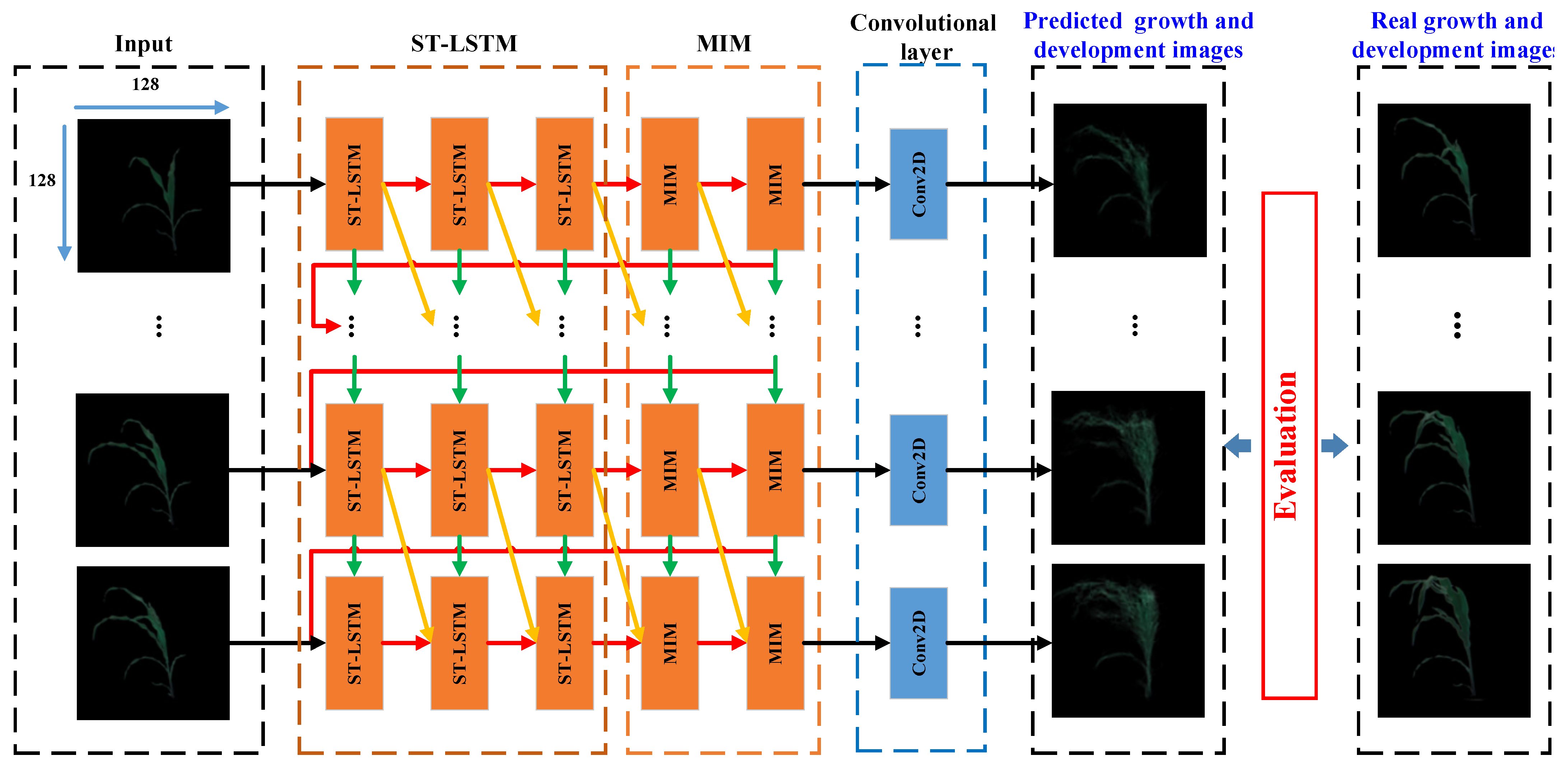
The prediction model of plant growth and development was trained on the training and validation dataset, and its performance was evaluated on the testing dataset. The proposed prediction model of plant growth and development consisted of one input layer, three ST-LSTM layers, two MIM layers, one convolutional layer, and one output layer. Three ST-LSTM layers were stacked and each contained 64 ST-LSTM units. Two MIM layers were stacked and each contained 64 MIM units. L2-Loss was chosen as the loss function, and Adam Optimizer with a learning rate of 0.001 was used in the loss function optimization. The batch size was set to two and the number of iterations was set to 80,000 for every training.
In order to validate the performance of the proposed prediction model, it was compared with the existing models, such as the prediction model based only on ConvLSTM [
5] and the prediction model based only on ST-LSTM [
13]. The comparison of evaluation results between the proposed prediction model and the existing models tested on the given dataset was conducted.
3.1. Successive-View Wheat Dataset
In the experimental study, the successive images of Fielder were firstly used to verify the effectiveness of the proposed prediction model. The sliding time window method was used to construct continuous time-series images as the input sequences of the model. The set window length slides along the time axis. The test dataset contained three waves of data (599 successive images at the middle growth stage, 144 successive images at the late growth stage, and 502 successive images at the mid to late growth stage) selected randomly from successive images of plant growth and development. The remaining successive images were considered for the training and validation dataset.
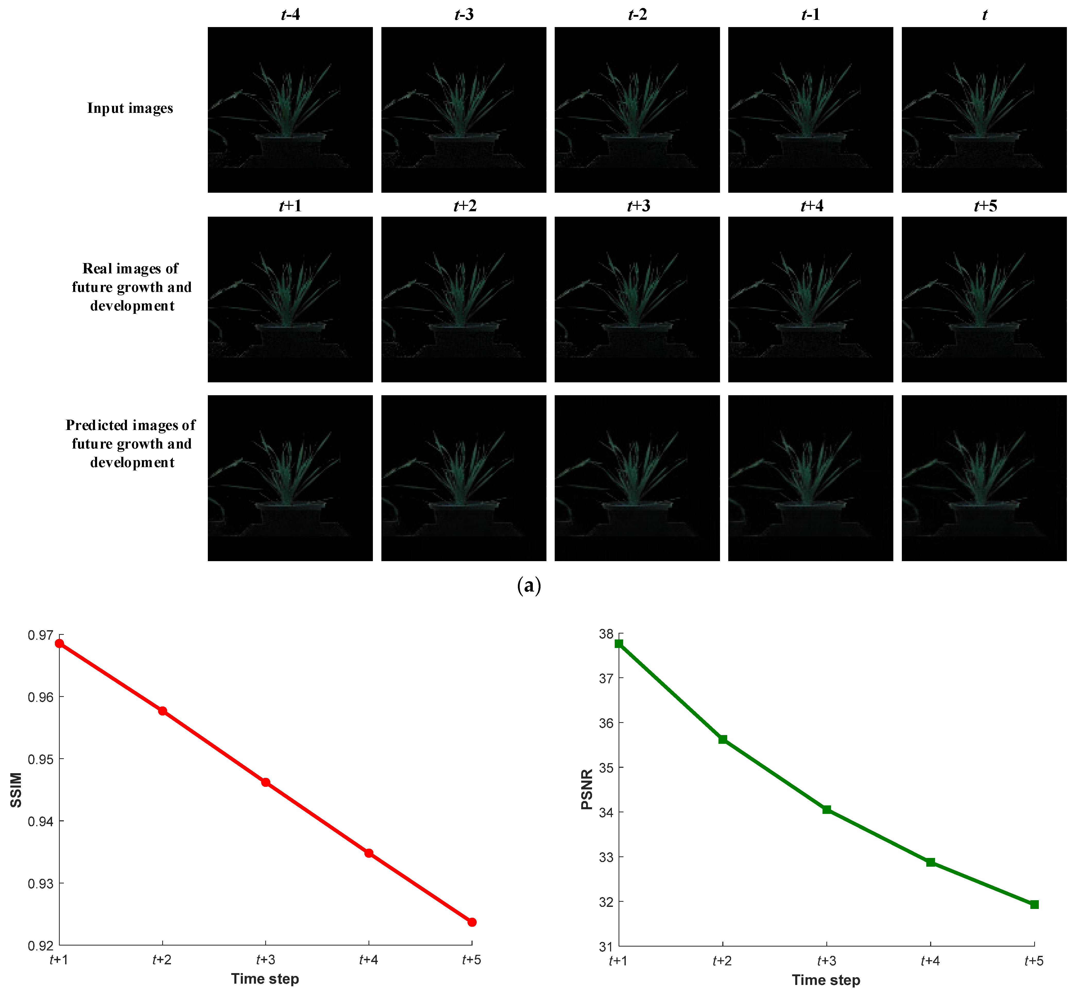
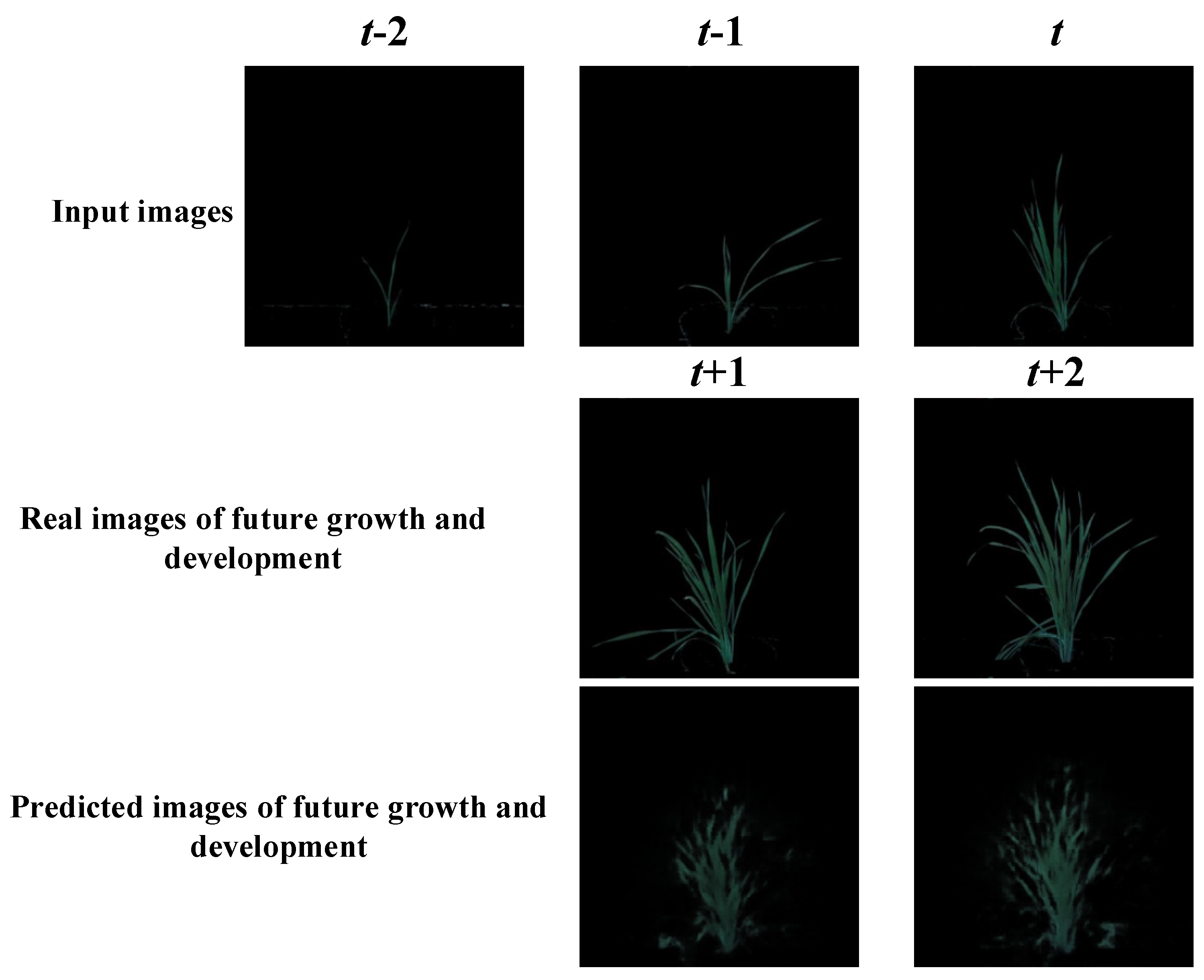
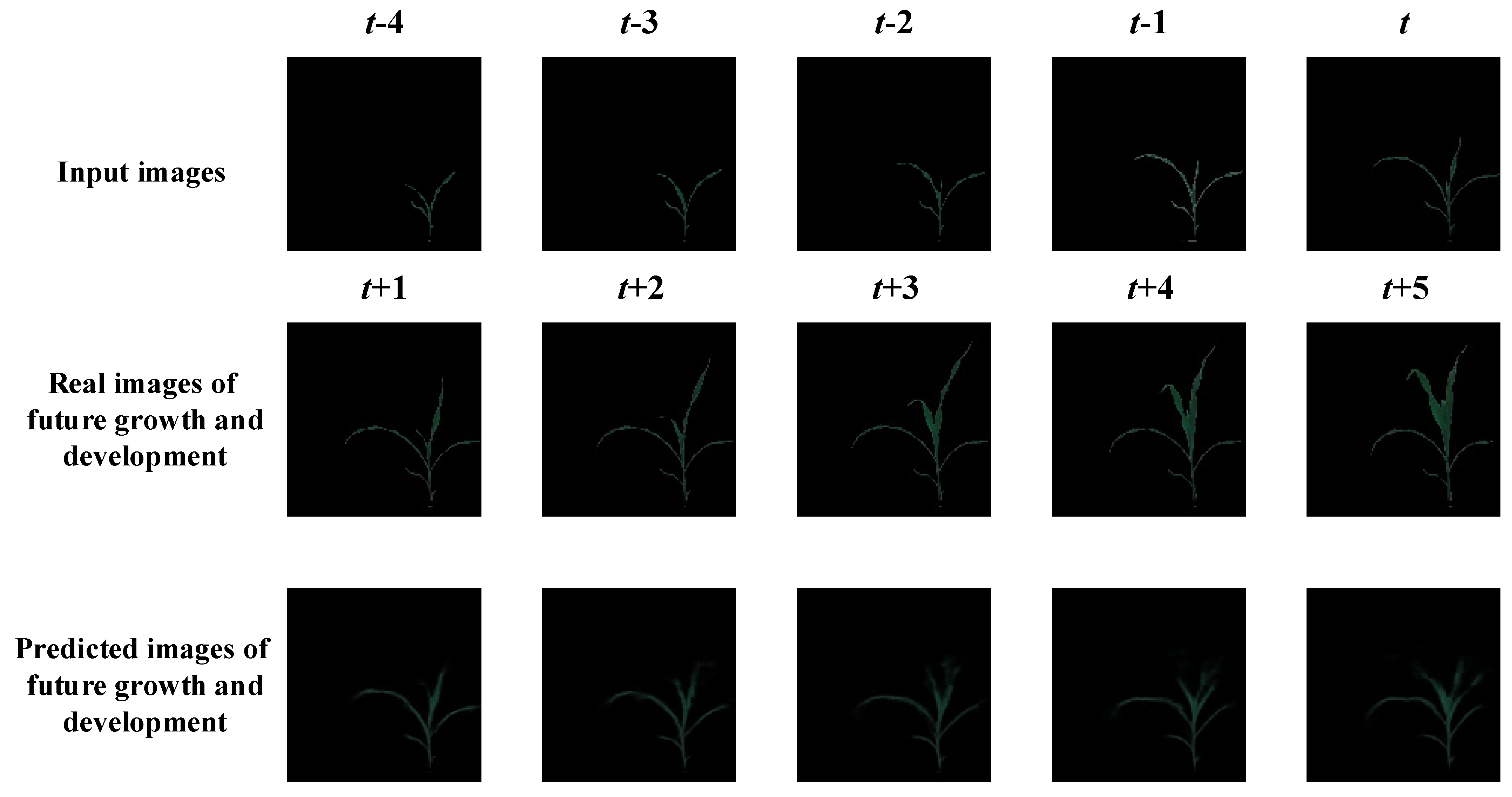
Five images of future growth and development were predicted at once based on five input images. The window length was set as 10. The prediction model was trained on the training and validation dataset and tested on the test dataset. The qualitative comparison between the predicted images and the real images of future growth and development is shown in
Figure 5a. The average values of MSE, PSNR, and SSIM at each step from
t + 1 to
t + 5 are shown in
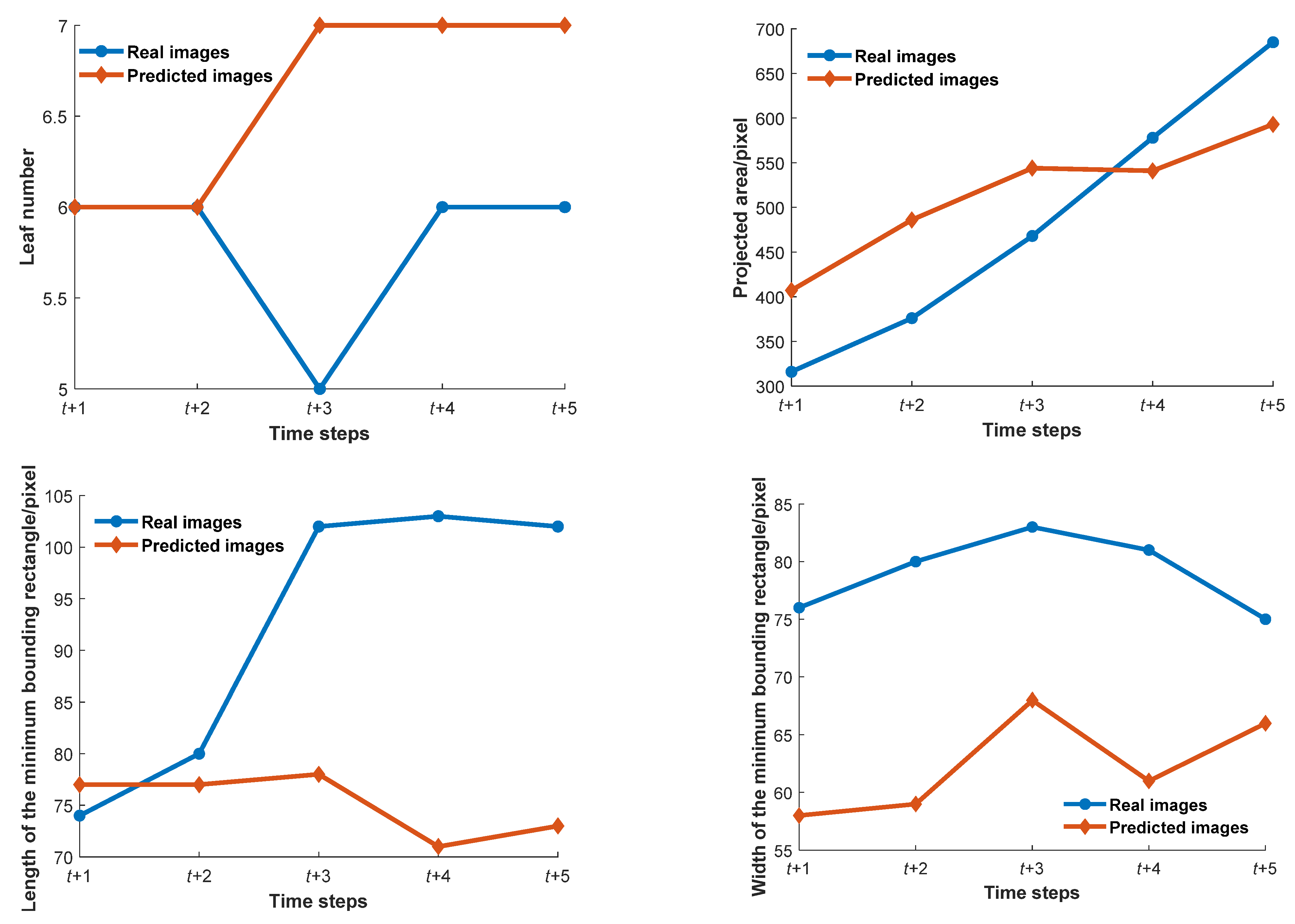
Figure 5b. The corresponding parameters (the leaf number, the projected area, and the length and width of the minimum bounding rectangle) of the predicted and real images were measured and compared, as shown in
Figure 5c.
The SSIM values surpassed 91% for all time steps. The mean of MSE values was 18.50 and the MSE values were below 30 for all time steps. The mean of PSNR values was 34.45. The smaller the value of MSE, the better the predictive ability of the proposed model. The results showed a high degree of similarity between the predicted images and the real images of plant growth and development. The values of PSNR and SSIM typically showed a gradual decrease trend as time step increased and the values of MSE showed a gradually increasing trend as time step increased. This may be caused by deviations of the predictions accumulated over time and the complexity of plant growth and development. Because the time interval between the two steps was only 30 min, the leaf number, and the length and width of the minimum bounding rectangle of real images had fewer changes and were similar to the ones of the predicted images, as shown in
Figure 5c. Yet, the rhythmic leaf movement and the growth of young leaves may change the projected area. There was a larger discrepancy between the projected area of predicted images and the projected area of real images. The changing trend of the projected area of predicted images is similar to that of real images. These results reflected the predictive validity of the proposed model.
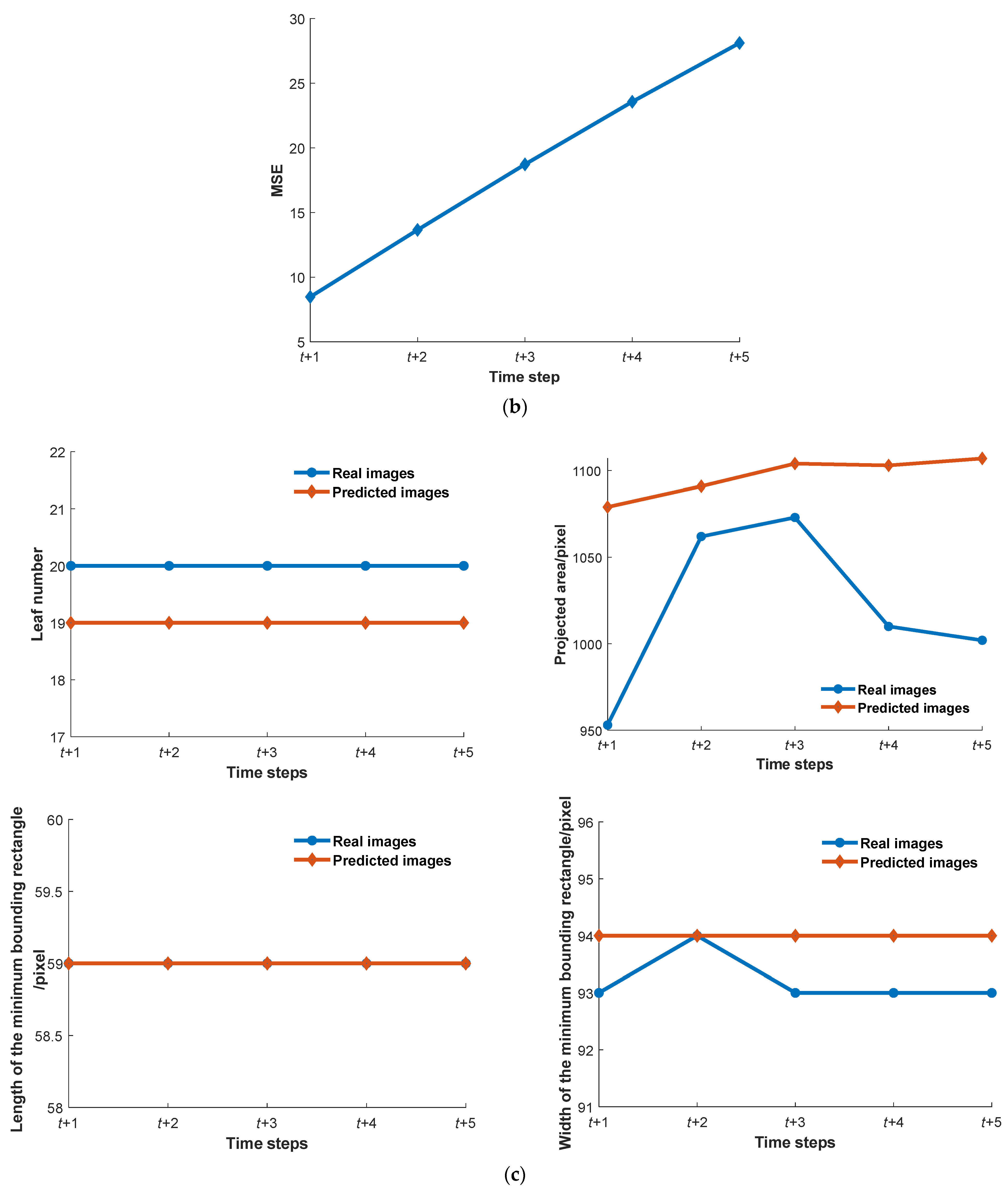
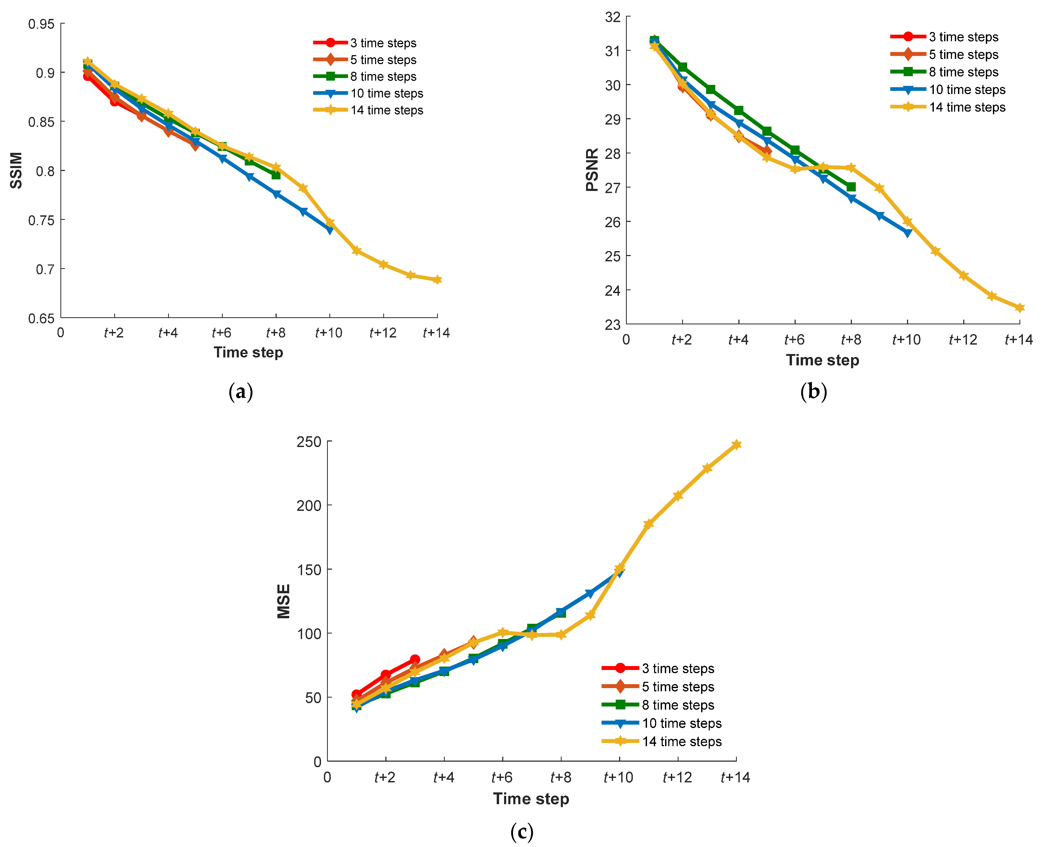
The prediction of plant growth and development at different numbers of time steps and different time intervals between two steps were compared to determine the optimal number of time steps and optimal time interval between two steps. The spacer input sequences of the model were acquired from the dataset at the set number of prediction steps and the time interval between time steps. The prediction results of different numbers of steps and different time intervals between steps are shown in
Figure 6.
The values of MSE, PSNR, and SSIM at each step between the predicted images with the real images are shown in
Figure 6, where the time interval between two steps was set as 30 min and the number of prediction steps was set as 3, 5, 8, 10, and 20. When the number of prediction steps was 20, the values of PSNR, and SSIM at each step were significantly lower than other results and the values of MSE at each step were significantly higher than other results. When the number of prediction steps was lower than 10, the values of MSE at each step (from
t + 1 to
t + 5) increased as the number of prediction steps increased (
Figure 6c), and the values of PSNR and SSIM at each step (from
t + 1 to
t + 5) were increased as the number of prediction steps increased (
Figure 6a,b). The standard deviations of MSE and PSNR values at each step were both less than two. The standard deviation of SSIM values at each step was smaller than 0.01. These results illustrate that the number of prediction steps had a comparatively small effect on the performance of the proposed prediction model until it was greater than 10.
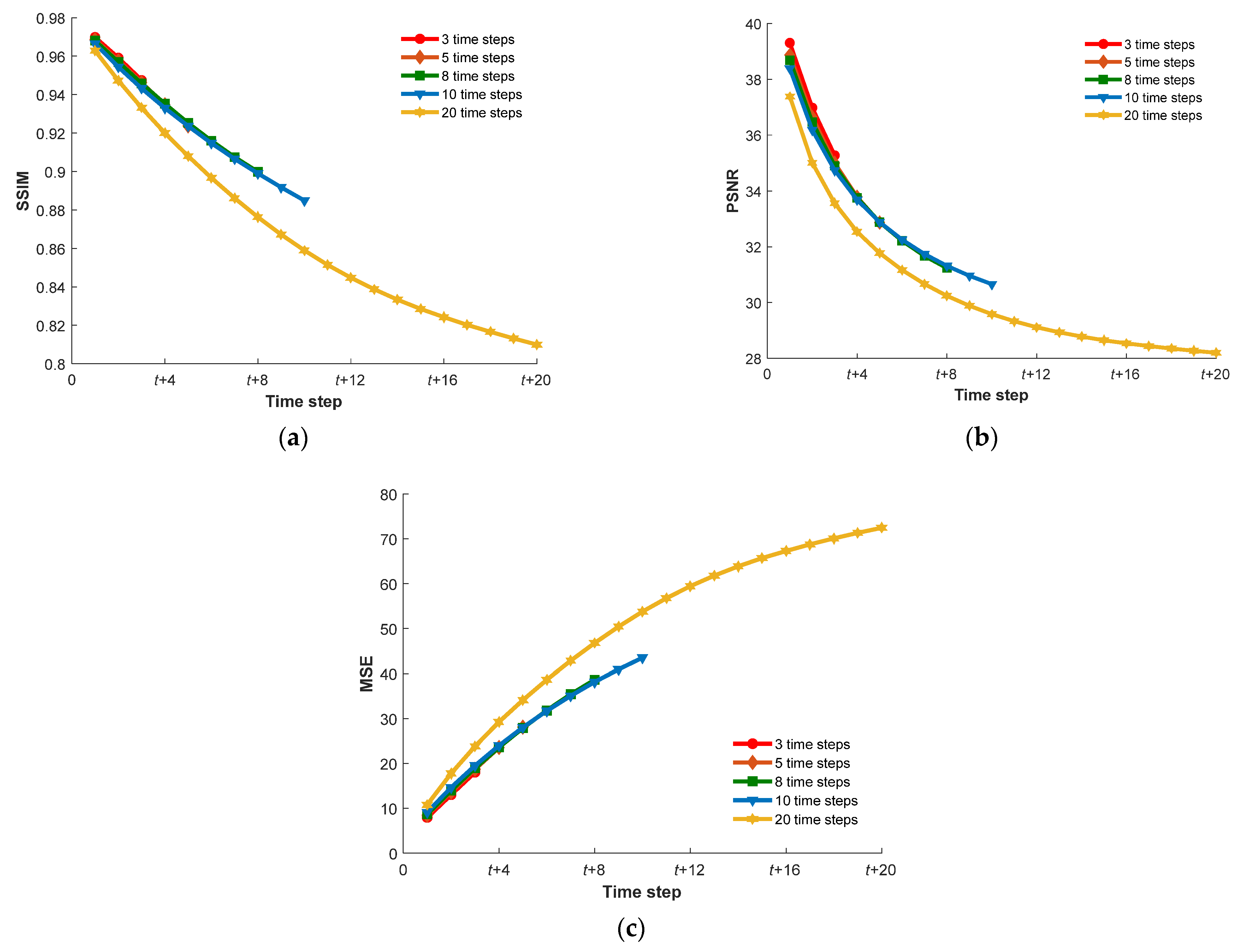
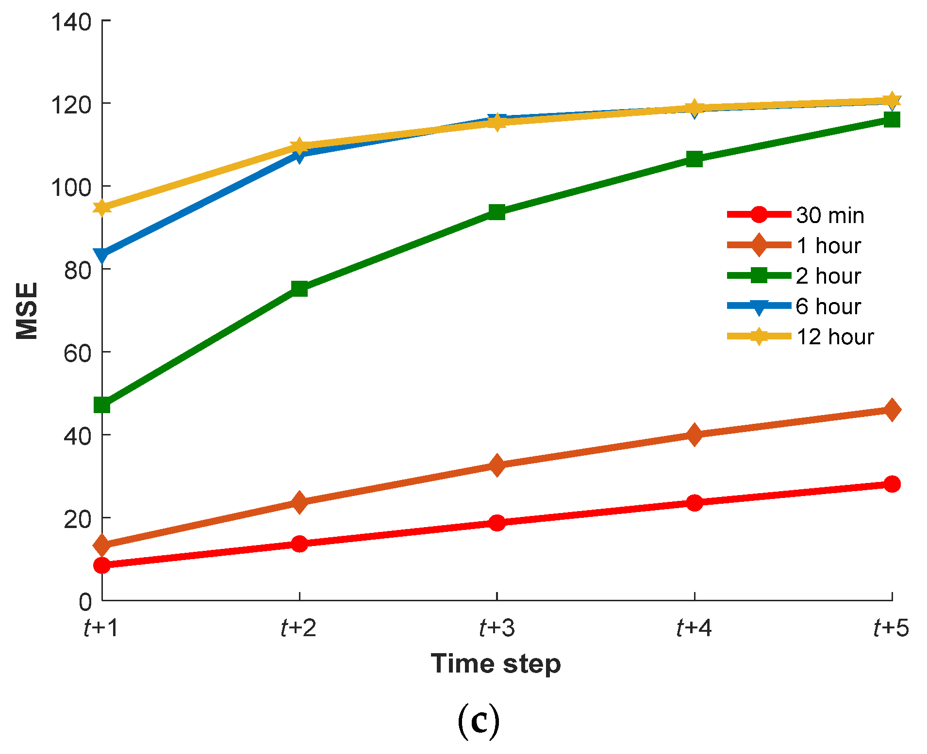
Next, the performances of the proposed prediction model tested on different time intervals were evaluated to explore the effect of the time interval between two steps on the proposed prediction model. The average values of MSE, PSNR, and SSIM at each step from
t + 1 to
t + 5 are shown in
Figure 7, where the time interval between two steps was set as 30 min, 1 h, 2 h, 6 h, and 12 h. The values of MSE at each step (from
t + 1 to
t + 5) were increased as the time interval between the two steps increased (
Figure 7c), and the values of PSNR and SSIM at each step (from
t + 1 to
t + 5) were increased as the number of prediction steps increased (
Figure 7a,b). However, when the time interval between the two steps was set as 2 h, the values of MSE at each step were significantly increased. When the time interval between the two steps was set as 6 h, the values of MSE at each step obtained were close to those obtained by setting the time intervals as 12 h. When the time interval between two steps was set as 6 h, the SSIM values surpassed 73% for all time steps and the SSIM value at the first time step was 79.85%, the mean of PSNR values was 26.68 and the mean of MSE values was 34.45. These results illustrate that the time interval had an extremely large effect on the performance of the proposed prediction model. In order to achieve 85% SSIM between the prediction and real plant images, the time interval needs to be set to 1 h. Therefore, for a more reliable and longer-term prediction of plant growth and development, the optimal number of time steps is 10 and the optimal time interval between two steps is 1 h.
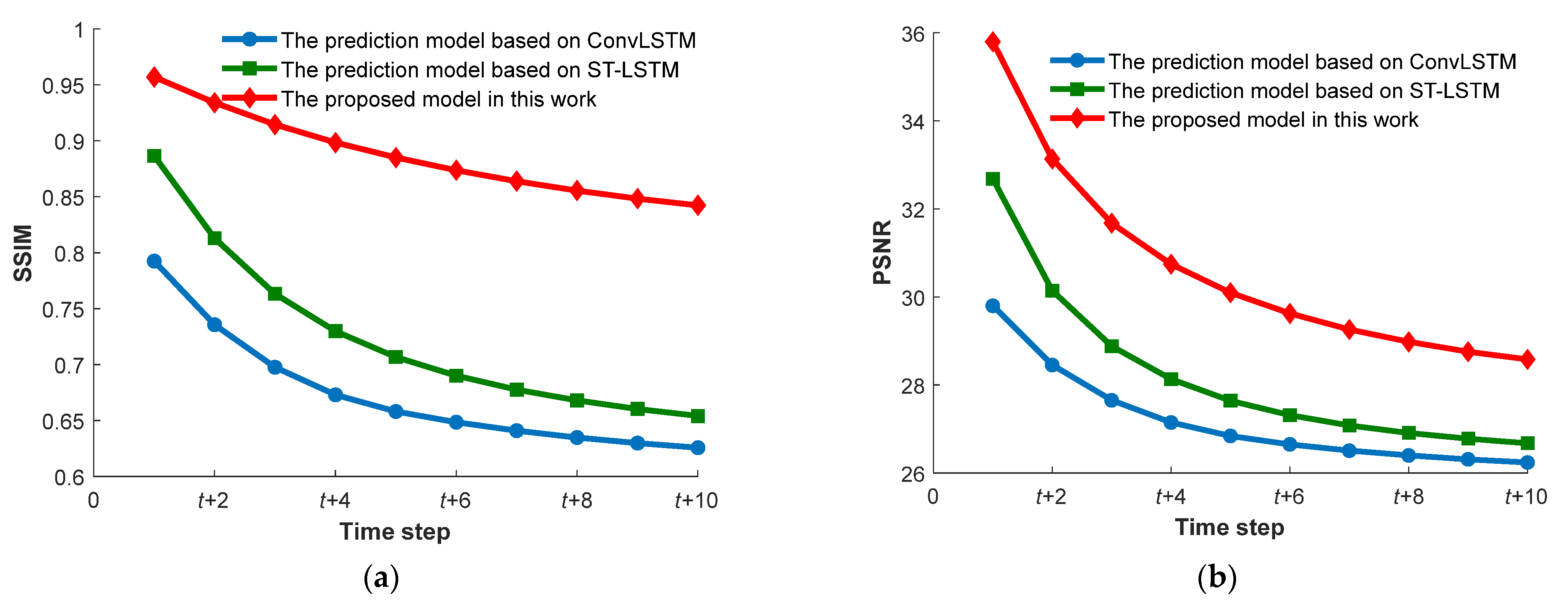
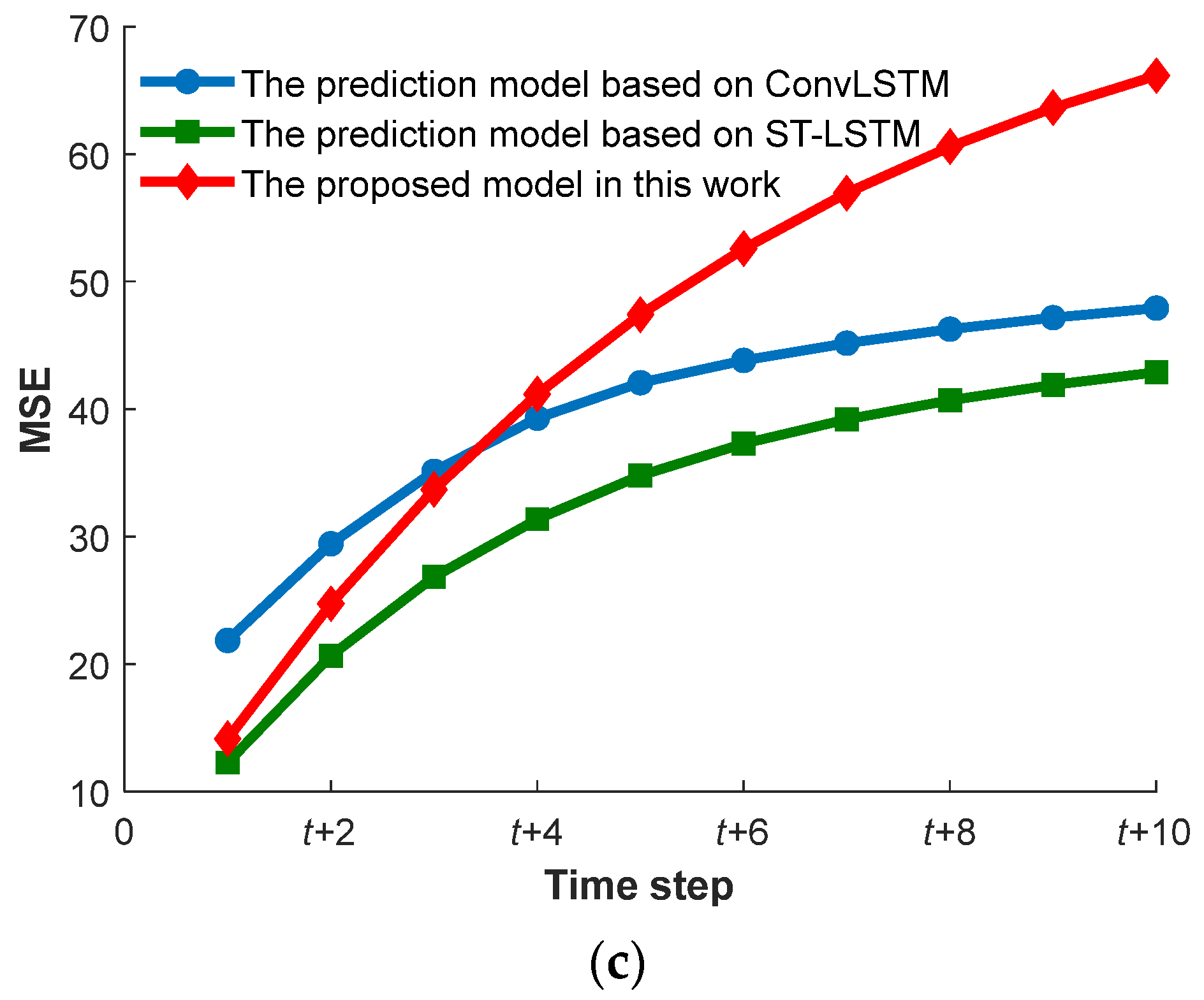
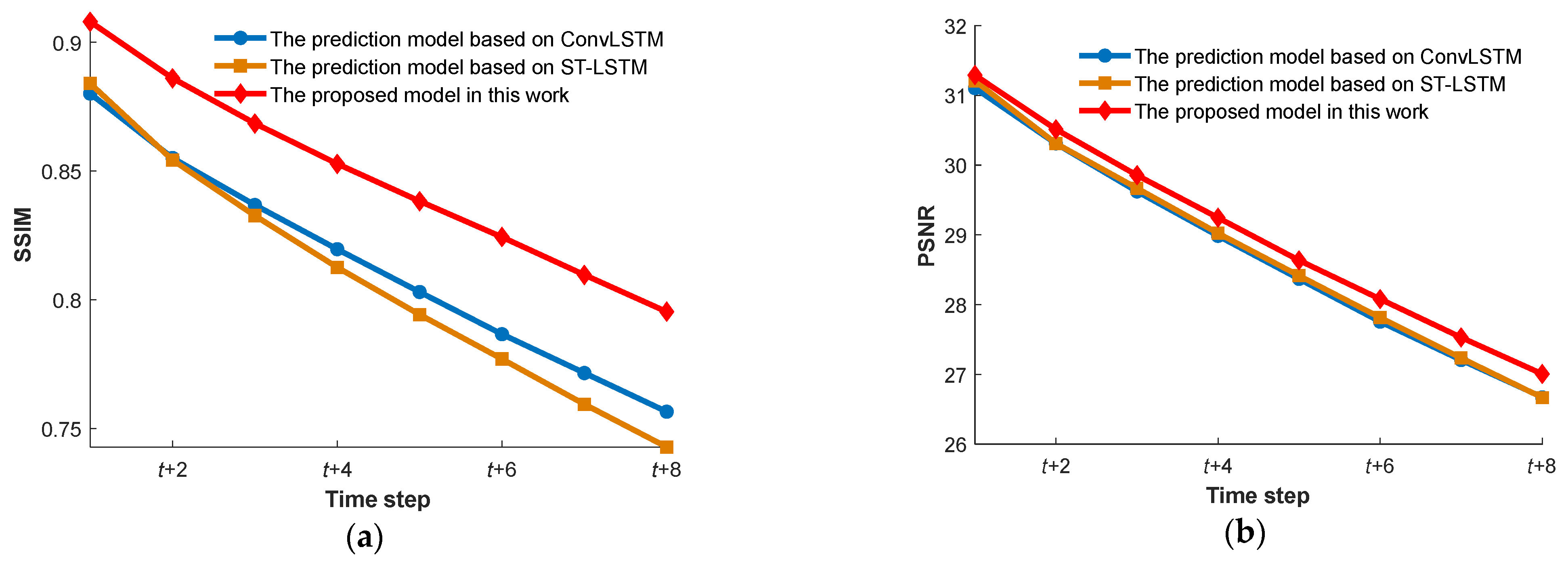
Under the optimal setting, the performance of the proposed prediction model and the existing models are shown in
Figure 8. The mean of PSNR values of the proposed prediction model was 30.67. The SSIM values of the proposed prediction model surpassed 85% for all time steps, which was higher than the ones of the prediction model based only on ConvLSTM and the prediction model based only on ST-LSTM. The mean of MSE values of the proposed prediction model was 46.11 and the MSE values of the proposed prediction model were below 68 for all time steps. The proposed prediction model was not good at the MSE. The MSE values of the proposed prediction model at each step (from
t + 4 to
t + 10) were higher than the ones of the prediction model based only on ConvLSTM and the prediction model based only on ST-LSTM. As shown in
Figure 5c, the projection area of wheat was as high as 1000 and the projection area was also the pixel number of the binary images. The relative difference of MSE between the proposed prediction model and the existing models was less than 30, which was acceptable. The results above validated the proposed prediction model and showed its robustness as compared with the existing models.
3.2. Multi-View Wheat Dataset
In the experimental study, the successive images of four different varieties of wheat without background were used to further verify the effectiveness of the proposed model in predicting the growth and development of different varieties and different views. The test dataset contained 144 sequences (obtained from eight views of 18 plants) selected randomly from the multi-view wheat dataset. The remaining sequences of successive images were considered for the training and validation dataset. The prediction model of plant growth and development was trained on the training and validation dataset. Two images of future growth and development were predicted at once based on three input images.
The proposed prediction model of growth and development was tested on the test dataset. The qualitative comparison between the predicted images and the real images of future growth and development is shown in
Figure 9. The average values of MSE, PSNR, and SSIM at each step from
t + 1 to
t + 2 were also calculated at different time steps to evaluate the predicted result of wheat growth and development. The values of SSIM at
t + 1 and
t + 2 steps were 81.63% and 80.46%. These results illustrate the validity of the proposed model again. When the time interval was increased, the predicted plant growth and development images could still have relatively good structural similarity with the real images by increasing the amount of training data.
3.3. Panicoid Phenomap-1 Dataset
The proposed prediction model was also evaluated on the Panicoid Phenomap-1 dataset. Successive images of 39 varieties of panicoid grain crops without background were used to verify the effectiveness and robustness of the proposed model in predicting growth and development. The test dataset contained 39 randomly chosen groups containing all genotypes of panicoid grain crops. The remaining 137 sequences of successive images were considered for the training and validation dataset. The prediction model was trained on the training and validation dataset and tested on the test dataset. Five images of future growth and development were predicted at once based on five input images. The window length was set as 10. The predicted images and the real images of future growth and development are shown in
Figure 10. The corresponding parameters (leaf number, projected area, length and width of the minimum bounding rectangle) of the predicted and real images were measured and compared, as shown in
Figure 11. The average values of MSE, PSNR, and SSIM at each step from
t + 1 to
t + 5 are also shown in
Figure 12.
The predicted results obtained by the proposed model on the Panicoid Phenomap-1 dataset were similar to the results above. The leaf number, projected area, and length and width of the minimum bounding rectangle of the predicted images were comparable and showed good agreement with the ones of real images. However, accuracies for late prediction time steps were lower, especially for the length of the minimum bounding rectangle. This problem is also reflected in the changing trend of the SSIM, MSE, and PSNR. When the number of time steps was set as five, the values of PSNR and SSIM typically decreased and the values of MSE increased with time. This again validated that the predicted results gradually become worse and may be caused by deviations of the predictions accumulated over time and the complexity of plant growth and development.
On the other hand, the number of prediction steps was set as 3, 5, 8, 10, and 20. The average values of MSE, PSNR, and SSIM at each step were also calculated to determine the optimal number of prediction steps, as shown in
Figure 12. The values of MSE at each step were first decreased and then increased as the number of prediction steps increased (
Figure 12c), and the values of PSNR and SSIM at each step were first increased and then decreased as the number of prediction steps increased (
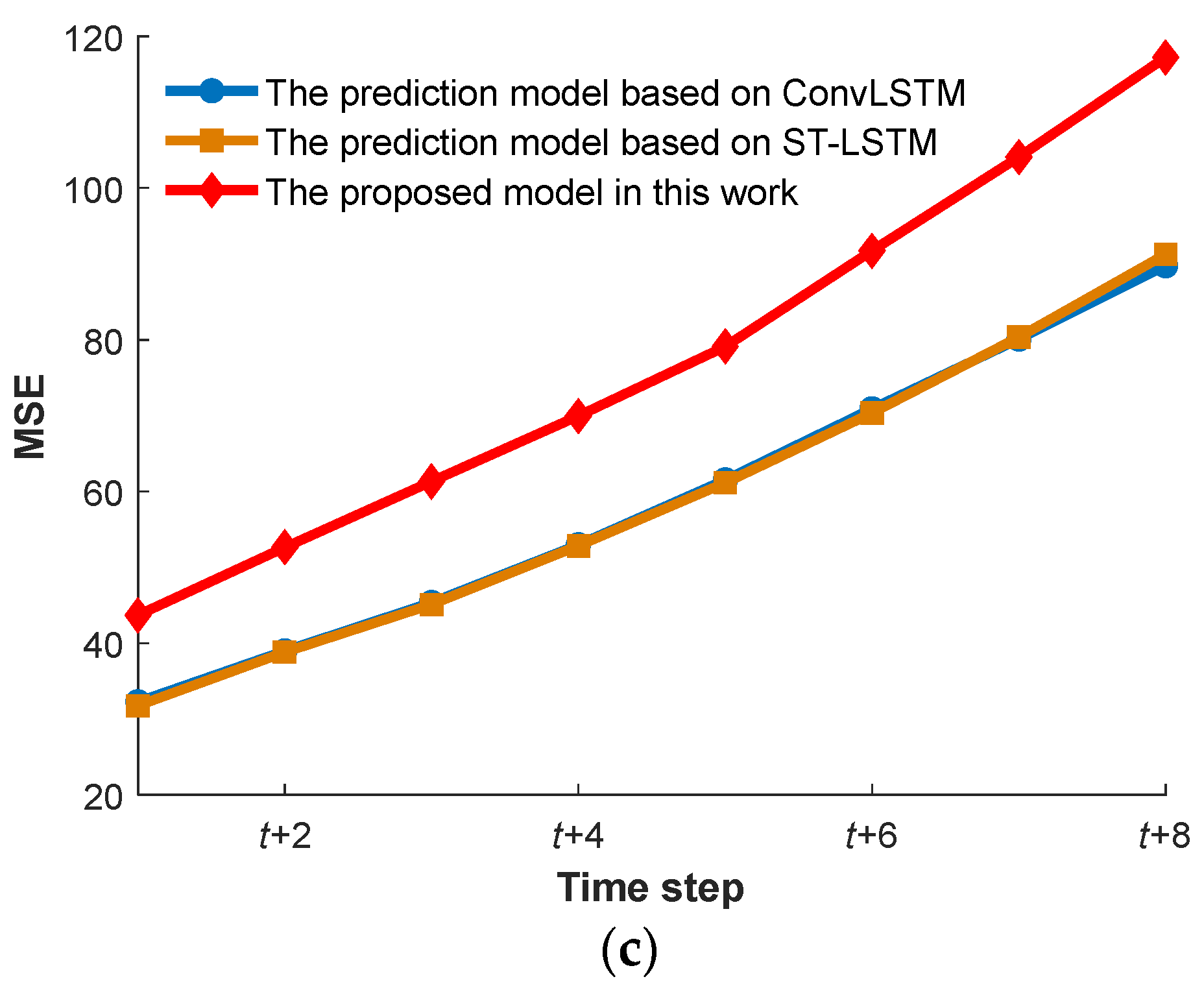
Figure 12a,b). The standard deviations of PSNR values at each step were less than two and the standard deviations of SSIM values at each step were smaller than 0.02. These results again illustrated that the number of prediction steps had a comparatively small effect on the performance of the proposed prediction model. However, a larger difference was found regarding the MSE values at each step obtained by setting different numbers of prediction steps. When the number of prediction steps was set to eight, the model had the best prediction performance on the Panicoid Phenomap-1 dataset. The SSIM values surpassed 78% for all time steps. The mean of MSE values was 77.78 and the MSE values were below 118 for all time steps. The mean of PSNR values was 29.03. The trend of the predicted results on the Panicoid Phenomap-1 dataset was different from that of the successive-view wheat dataset. This may be caused by the increase in the time intervals. The time intervals between two steps of the successive-view wheat dataset were less than 12 h. The real images of plant growth and development at the time step
t + 1 bore a strong visual resemblance to the real images at the time step
t + 1. However, the time interval of the Panicoid Phenomap-1 dataset was 24 h. With the number of prediction steps increased, the proposed model can better model the dynamic of plant growth and development to predict plant future growth and development. In parallel, deviations of the predictions accumulated over time became more conspicuous. Therefore, when the number of prediction steps was set to eight, the model had the best prediction performance on the Panicoid Phenomap-1 dataset.
Under the optimal setting, the performances of the proposed prediction model and the existing models are shown in
Figure 13. The SSIM and PSNR values of the proposed model are significantly higher than those of the prediction model based only on ConvLSTM and the prediction model based only on ST-LSTM. The proposed prediction model was also not good at the MSE. The results were similar to the results above. The MSE values of the proposed prediction model at each step were higher than the ones of the prediction model based only on ConvLSTM and the prediction model based only on ST-LSTM. The relative difference of MSE between the proposed prediction model and the existing models was less than 40. These results above again validated the robustness of the proposed prediction model.
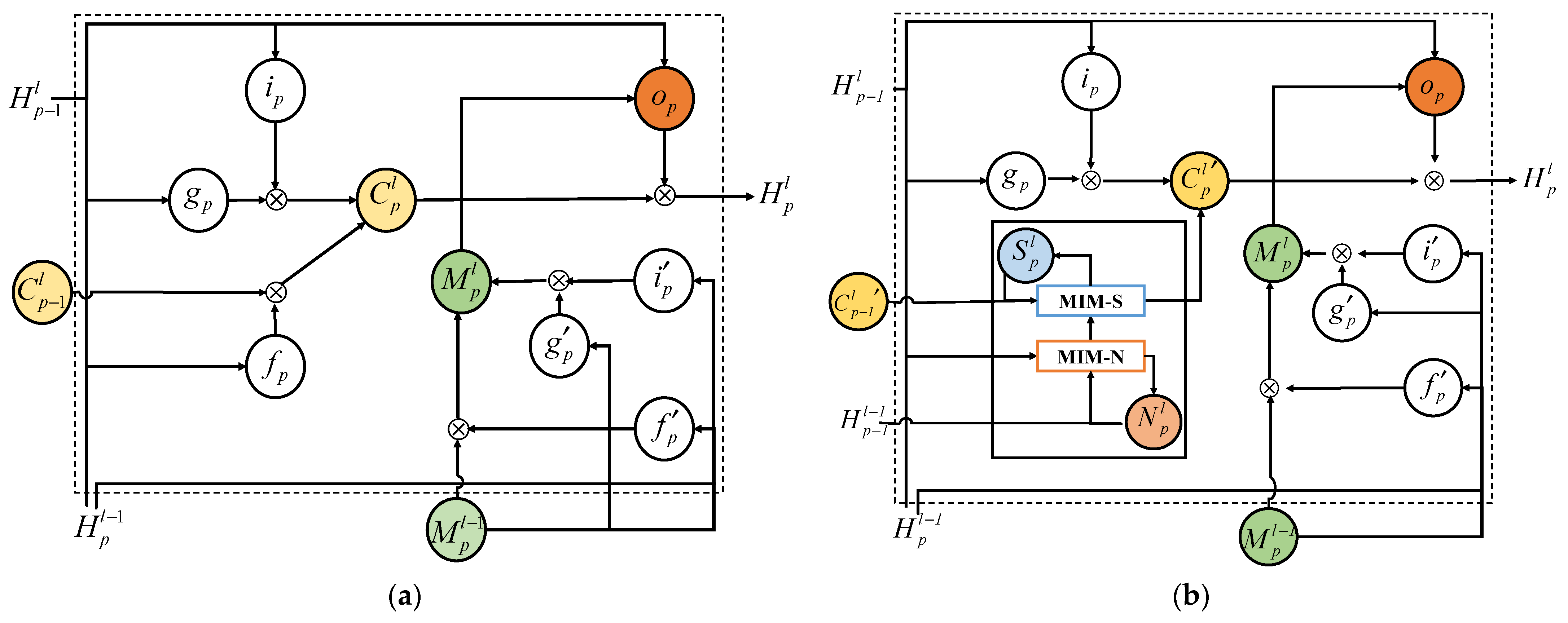
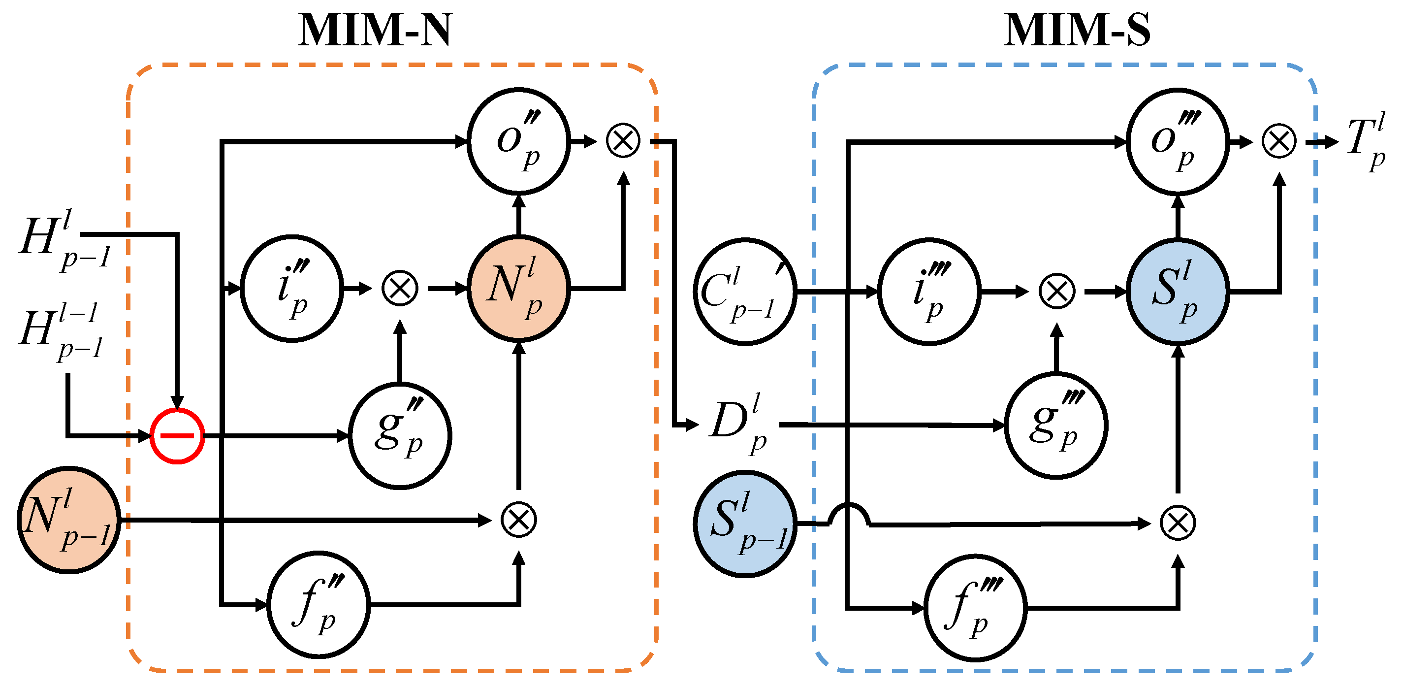
Compared with others’ work using GAN models, the proposed model did not perform well in terms of the blurriness of the predicted images. Nevertheless, there are two advantages of this work. The first advantage is that the images of future plant growth and development predicted by the proposed model have higher structural similarities with the real images. The proposed model predicted the future images of plant growth and development by modeling the dynamic behaviors of plant growth and development using ST-LSTM and MIM modules. The hidden presentations of spatiotemporal stationarity variations in the time-series images were generated by the ST-LSTM layers. The MIM exploits the differential signals between adjacent recurrent states to model the non-stationary and approximately stationary properties in spatiotemporal dynamics with two cascaded, self-renewed memory models. By stacking multiple MIMs, we could potentially handle higher-order non-stationarity of plant growth and development. The second advantage is that the effect of the number of time steps and the optimal time interval between two steps on the prediction performance of the proposed model was analyzed and the optimal number of time steps and the optimal time interval between two steps were determined, which will provide a valuable reference for the prediction studies of plant growth and development.


 and
and 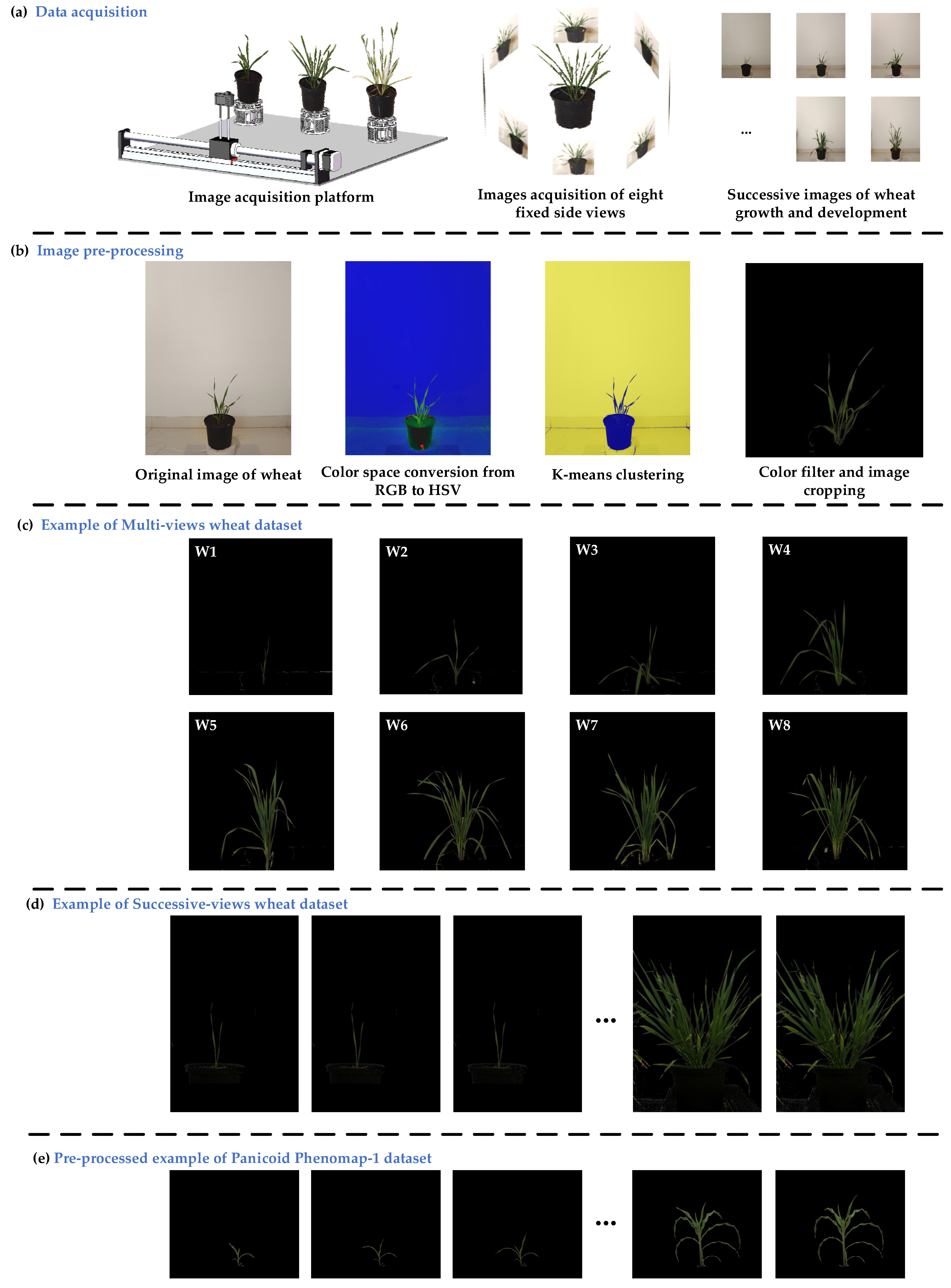


