The first results presented refer to studies carried out to determine the spatial and temporal discretization to be adopted and to verify the numerical model used to generate the waves. Then, the results related to the geometric optimization of the obstacle coupled to the overtopping wave energy converter, the main objective of the present study, are presented.
4.1. Mesh and Time Step Independence Study and Verification of the Computational Model
It is worth mentioning that the mesh used was composed of regular rectangles. This kind of finite volume has the advantage of avoiding numerical effects such as false diffusion on the solution of the primary variables of the problem, which could occur by using an irregular mesh with triangular volumes. Thus, in this study, a mesh convergence test was carried out, simulating four cases with a different number of volumes, 19,000, 38,000, 76,000, and 152,000. The results were compared with the calculation of the analytically generated wave (Equation (9)). Therefore, the elevation of the free surface was monitored using a numerical probe of the integral type located at x = 50.00 m.
Furthermore, for the mesh independence test, a time step of ∆t = 2.00 × 10
−2 s was considered.
Table 5 shows the MAE average, calculated using Equation (15), and the processing time demanded for each simulation for different meshes investigated.
To determine the best mesh, the refinement and processing time of the simulation were considered along with the calculated numerical error. After verifying that the difference between a mesh of 76,000 and one of 152,000 volumes is only 0.01%, lower than the difference observed in the other cases analyzed, a mesh with 76,000 regular rectangular volumes was then adopted.
Since it is a transient problem, the temporal discretization employed was defined by carrying out a time step independence study. For this study, four simulations are performed considering a total time of wave flow over the overtopping device of 100 s and varying the time step by: ∆t = 5.00 × 10⁻³ s, ∆t = 1.00 × 10⁻² s, ∆t = 2.00 × 10⁻² s, and ∆t = 4.00 × 10⁻² s.
Table 6 presents the free surface elevation values (
η) obtained at
x = 50.00 m and for the instant of time
t = 15.00 s for each time step studied and the variation among the tested cases. Consequently, the time step of ∆
t = 2.00 × 10
−2 s was adopted for the geometric evaluation simulations since it leads to less computational effort among the best time steps. Moreover, only the time step ∆
t = 2.00 × 10
−2 s has a higher discrepancy in the magnitude of
η compared to the other investigated time steps.
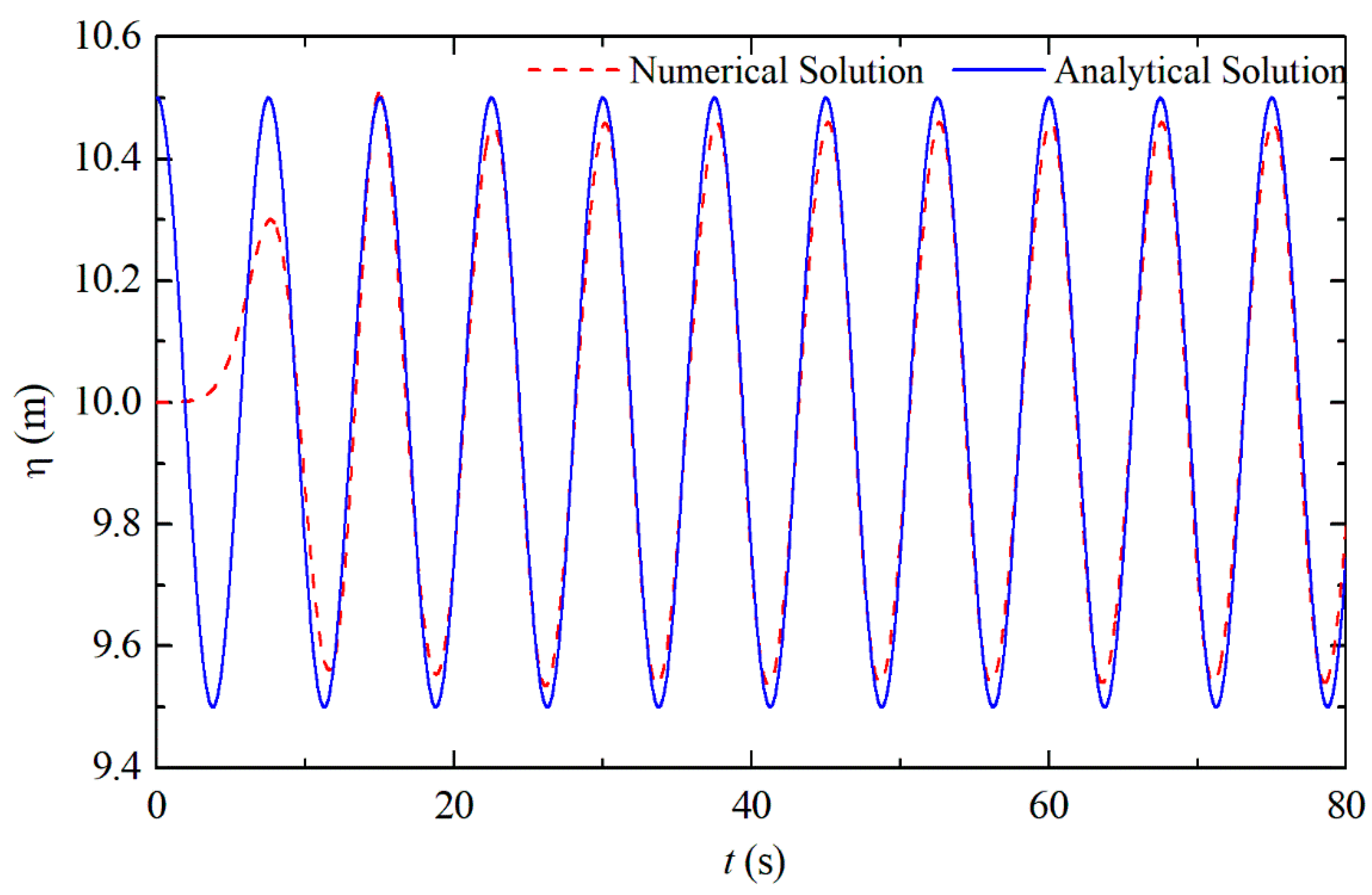
The analytical solution (Equation (9)) was compared to the numerical solution for a wave generated in a channel without the device to verify the methodology employed. This comparison is presented in
Figure 5, where it is possible to verify that the numerical wave fits well in the analytical solution for
t > 15.00 s where the stabilization occurred. Before this period, the numerical solution is influenced by the initial condition of inertia of the flow, which is not contemplated in the analytical solution. Thus, the wave generation verification considered the interval of 15.00 s ≤
t ≤ 80.00 s.
Evaluating the difference between the analytical and numerical results, when calculating the MAE comparing the elevation of the free surface in the wave channel, considering the depth of h = 10.00 m, a result of approximately 0.10% was obtained. However, when calculating the average MAE considering only the generated wave, i.e., disregarding the water depth on the channel, an average of 8.00% was obtained. Thus, there is a good agreement between the results.
It is also worth mentioning that a validation of the present computational method was performed in a previous research group work. A comparison between the free surface elevation as a function of time in a laboratory-scale wave channel obtained with the present computational model and those obtained experimentally in the work of Goulart [
45] was performed.
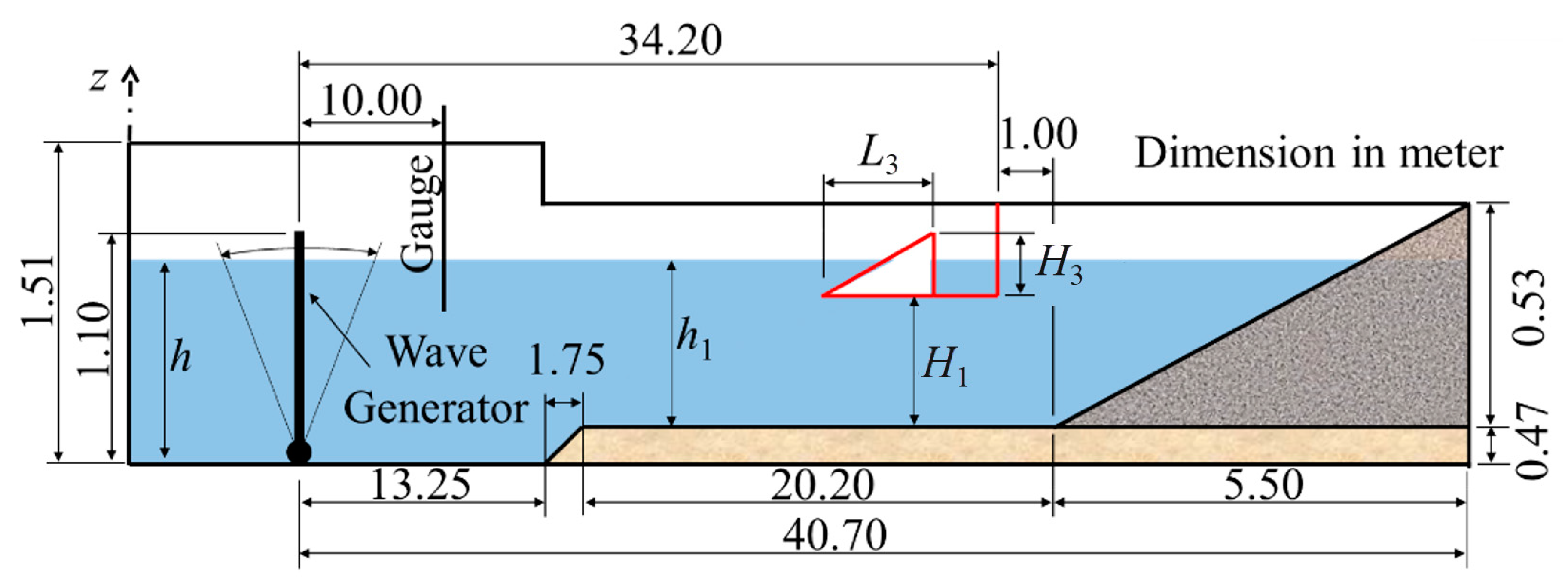
Figure 6 illustrates the wave channel at a laboratory scale used in the work of Goulart [
45], which was reproduced numerically with the present computational method. The following dimensions were adopted in the problem:
LT = 34.2 m,
HT = 1.0 m,
H1 = 0.15 m,
Lr = 0.5 m,
h = 0.862 m,
h1 = 0.392 m,
H3 = 0.279 m, and
L3 = 0.716 m, leading to a ramp angle of 21.3°. Moreover, it is considered that the waves reaching the device have a period of
T = 1.94 s, height of
H = 0.067 m, and wavelength of
λ = 3.54 m.
Figure 7 shows the results of the height of water accumulated in the reservoir as a function of time obtained in the experiment of Goulart [
45] (red line) and the numerical predictions obtained with the present computational method (black line). As can be observed, the experimental and numerical results were in close agreement, with a difference of 1.8%. The numerical results also predicted the beginning of the overtopping occurrence (
t~22.5 s) and the slope of the curve of water accumulation in the reservoir well. Therefore, it is possible to state that the present computational method is verified and validated.
4.2. Geometric Investigation of the Overtopping Device with Coupled Obstacle
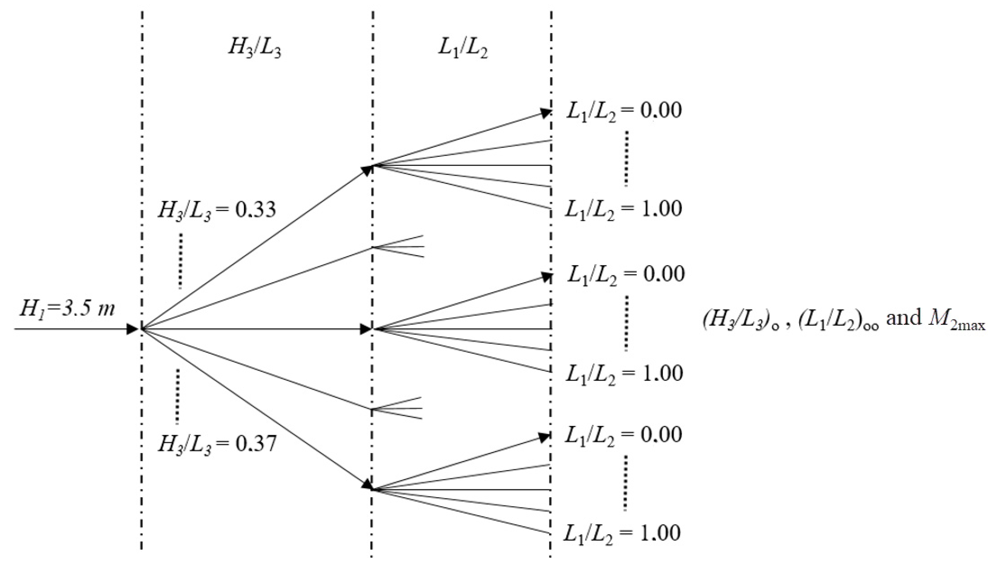
To perform the geometric evaluation, the geometry of the overtopping device with five different
H3/
L3 ratios, previously studied in [
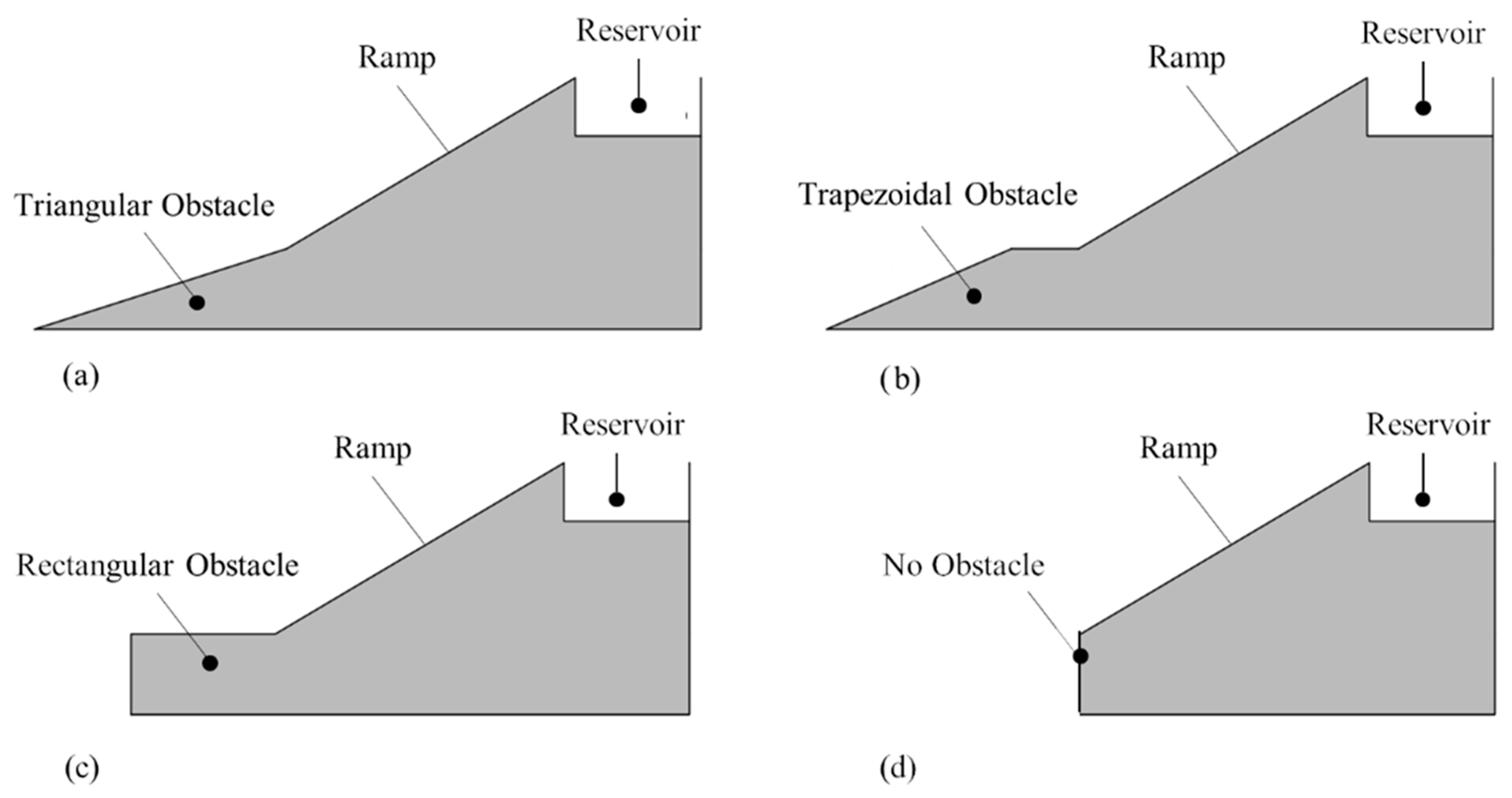
24], is considered. The obstacle attached to the device varied between the lowest magnitude of
L1/
L2 = 0.00, representing a triangular configuration, and the highest magnitude of
L1/
L2 = 1.00, representing a rectangular configuration. Intermediate ratios of
L1/
L2 (0.00 <
L1/
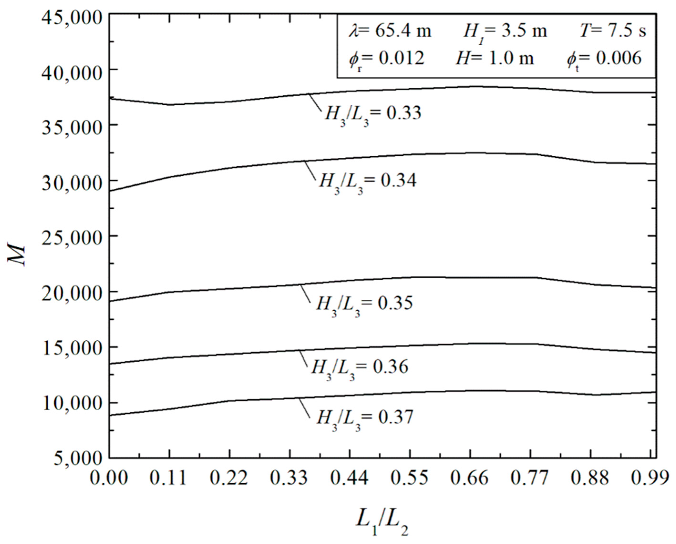
L2 < 1.00) refer to trapezoidal obstacles. The total sum of the mass of water entering the reservoir over the 100.00 s simulated was calculated to compare the performance of the different geometries.
Figure 8 shows the effect of the ratio
L1/
L2 over the total amount of water mass accumulated in the reservoir over the time interval considered (
M) for different values of
H3/
L3. It is possible to observe that the ratio
H3/
L3 = 0.33 conducted to the maximum water accumulation in the reservoir was almost
M = 40,000 kg, while ratios of
H3/
L3 = 0.37 led to an amount of mass in the range of
M = 10,000 kg, i.e., a ratio of 4.5 times between the best and worst conditions of
H3/
L3. Results also indicated that the effect of
L1/
L2 on the device performance was significantly lower than the effect of
H3/
L3 over
M, i.e., the sensibility of
H3/
L3 was much higher than
L1/
L2 over the overtopping performance. One example can be noticed for
H3/
L3 = 0.33, where the difference between the best configuration of
L1/
L2, (
L1/
L2)
o = 0.67 led to a performance of only 5.00% superiority to that achieved for the worst configuration (
L1/
L2 = 0.11). As the magnitude of the ratio
H3/
L3 increases, the influence of the ratio
L1/
L2 over
m increases, as can be attested for the ratio
H3/
L3 = 0.37, where the best configuration of
L1/
L2, (
L1/
L2)
o = 0.67 conducted a performance nearly 20.00% superior than the triangular configuration (
L1/
L2 = 0.00) which conducted to the worst performance. Moreover, for all cases using
H3/
L3 an optimal intermediate configuration of
L1/
L2 is obtained. Despite presenting a secondary contribution, the ratio
L1/
L2 improved the overtopping device, mainly for non-optimized ratios of
H3/
L3.
The best configurations found in
Figure 8 are summarized in
Figure 9, presenting the effect of the ratio
H3/
L3 over the once-maximized mass of water accumulated in the reservoir,
Mmax. The results reinforced the strong sensitivity of the ratio
H3/
L3 over the overtopping device performance. It is also noticed that, for almost all cases, the ratio
L1/
L2 = 0.67 led to the best performance, except for the case with
H3/
L3 = 0.35, where the ratio
L1/
L2 = 0.54 was the best. Thus, the
L1/
L2 ratio that provides the best performance in all cases has a trapezoidal shape. When considering a triangular obstacle,
L1/
L2 = 0.00, the wave flow suffers a dispersion and the overtopping is not favorable, i.e., the configuration of the ramp and obstacle acts as a beach, smoothing the intensity of the wave that reaches the final stage of the ramp. On the other hand, considering a rectangular obstacle,
L1/
L2 = 1.00, there is a greater reflection of the wave, also disfavoring the intensity of the flow that reaches the ramp.
The fluid dynamic behavior of the problem is shown, for some instances of time, in
Figure 10 and
Figure 11, where the water volumetric fraction and velocity fields are displayed. Thereby, it is possible to observe how the wave flows over the device for the case with the optimal ratio of (
H3/
L3)
o = 0.33, considering three different obstacle ratios, (a)
L1/
L2 = 0.11, (b) (
L1/
L2)
oo = 0.67, and (c)
L1/
L2 = 1.00. Furthermore, in
Figure 10, water is represented by red, while air is represented by blue. Through the volume fraction fields in
Figure 10, it is possible to observe the overtopping occurrence in the instances of time
t = 74.00 s and 75.00 s for different configurations of
L1/
L2 investigated. In all plotted cases, between the time instances of 73.00 s ≤
t ≤ 75.00 s, it is observed that the water mass generates a high inflection in the free surface, which leads to a wave-breaking process, causing the overtopping. From
t = 76.00 s on, it is noted that the wave stabilizes and the mass of water begins to move in the opposite direction, towards the base of the ramp. In
Figure 11, among the color scales, red represents higher velocities while blue represents the lower ones. In all situations, it is observed that the highest magnitudes occur in the air due to the lower air density. In the time interval 74.00 s ≤
t ≤ 75.00 s, the mass of water entering the reservoir causes a boundary layer detachment, increasing the magnitude of velocity fields even more in the airflow near the water jet entering the reservoir. In the water region, the highest magnitudes can be noticed when the wave is in the imminence to overtop the ramp and after the overtopping, when the water is in the opposite direction of the wave flow. In this situation, the water going down the ramp meets the next incident wave, generating a mixture of streams and intensifying the velocity magnitude. Concerning the comparison of ratios
L1/
L2, only slight differences are observed in the volume fraction and velocity fields, which are reflected in the small differences found between the best and worst configurations.
Finally, a comparison among three different configurations coupled with the overtopping device was performed: 1—trapezoidal for the optimal ratio of
L1/
L2, 2—rectangular (
L1/
L2 = 1.00), 3—triangular (
L1/
L2 = 0.00), and one configuration without a seabed structure (for the same conditions studied in the work of Martins et al. [
25]).
Figure 12 illustrates the effect of the ratio
H3/
L3 over the amount of mass overtopped in the reservoir (
M) along the time interval for the four studied configurations. It is important to mention that the mass accumulated in the reservoir is directly proportional to the potential energy of water in the device, considering the use of the same reservoir for all investigated configurations, as is the case here. Therefore, the highest magnitudes of
M led to the highest energy conversion when the water in the reservoir is expanded in a low-head turbine. Results demonstrated that the best configuration is the trapezoidal, followed by the rectangular and triangular configurations, respectively, regardless of the ratio
H3/
L3. Moreover, results demonstrated that the differences between the different configurations with the coupled structure are not significant, mainly for (
H3/
L3)
o = 0.33, where differences are nearly 4%. Despite the influence of the degree of freedom of
L1/
L2 being smaller than that of
H3/
L3, analyzing the results shown in
Figure 12, it is possible to state that the configuration of the obstacle-ramp set captures a greater amount of water mass in the reservoir, making this configuration more efficient compared to the conventional overtopping device. For the twice optimal configuration, i.e., for (
H3/
L3)
o = 0.33 and (
L1/
L2)
oo = 0.67, the coupling of the trapezoidal structure improved the device performance by 30% when compared to the conventional device for the same
H3/
L3 ratio. For non-optimized ratios of
H3/
L3, the influence of the seabed structure is even more important. For instance, for
H3/
L3 = 0.34, the performance reached with the trapezoidal structure is around 1.7 times superior to the case without the structure.


 ,
, 


