Dynamically-Tunable Dataflow Architectures Based on Markov Queuing Models

Abstract

Dataflow architectures are fundamental to achieve high performance in data-intensive applications. They must be optimized to elaborate input data arriving at an expected rate, which is not always constant. While worst-case designs can significantly increase hardware resources, more optimistic solutions fail to sustain execution phases with high throughput, leading to system congestion or even computational errors. We present an architecture to monitor and control dataflow architectures that leverage approximate variants to trade off accuracy and latency of the computational processes. Our microarchitecture features online prediction based on queuing models to estimate the response time of the system and select the proper variant to meet the target throughput, enabling the creation of dynamically-tunable systems.

1. Introduction

Modern applications require the elaboration of massive amounts of data, e.g., in realtime video streaming for entertainment or surveillance applications, or network communications [1,2]. To achieve high performance, such applications demand heterogeneous System-on-Chip (SoC) architectures with specialized hardware components. Thanks to customization, these architectures can significantly minimize the cost, while hardware parallelism can optimize the execution time [3].

Due to their distributed nature, modern applications may need to support variable behavior, where input data are not always available at the same speed [4]. In such cases, designers must guarantee not only a high quality of the result (e.g., a nice video experience) but also a continuity of the service (e.g., continuous streaming in surveillance). Latency-insensitive protocols can be used to ensure correct execution in case of changes in the surrounding behavior, for example by stalling the execution of the component when the data are not available [5]. However, hardware accelerators have limited flexibility. Their entire behavior must be defined and implemented at design time. After that, they cannot implement a new functionality. Furthermore, the execution time is fixed and depends on the microarchitecture. In case of variable behaviors, one can design the components considering the fastest speed that can support all behaviors (“worst-case” approach) but the resulting component would be underutilized in most of the cases or can even create congestion on the next components, since it produces the results too fast. Targeting an average speed, instead, would lead to congestion on the inputs when the component cannot keep pace with the input data. These situations have been exploited to reduce the power consumption with dynamic frequency and voltage scaling (DVFS) [6]. and they can also be used for implementing adaptive behaviors.

In software, designers can achieve adaptivity by approximating the execution of some phases, provided that the application designers can accept a minimal degradation of the outputs [7]. When multiple approximate alternatives are available for the same code, the system can select dynamically which version to be executed. Such systems are called multi-variant [8]. When applied to hardware, approximation can either save resources (i.e., less logic is used to perform the same computation) or improve the performance (i.e., some computation can be executed faster, improving the hardware microarchitecture or performing the operations in a different way). While many software approximation techniques can be easily applied to hardware accelerators (e.g., variable-to-constant optimizations [9]), multi-variant hardware systems are more difficult to be designed since they need to (1) design efficient hardware modules able to support all variants and (2) detect the proper variant efficiently and correctly based on the given workload.

In this paper, we focus on the second aspect of the problem, assuming that the designer applies existing approximation techniques to generate multi-variant hardware components. With our control approach, we enable the creation of dynamically-tunable dataflow architectures by managing multi-variant accelerators that can dynamically adapt their execution speed to the surrounding conditions. This system allows modulating the hardware to use the approximate versions of a given functionality only when strictly necessary. We start from components that implement multiple variants trading off accuracy and latency. Such variants (also called configurations) can be generated with different approximation solutions and merged to reduce area overhead. We extend the multi-variant hardware module with a microarchitecture to automatically select the proper configurations based on the system workload. Such microarchitecture monitors the input data, estimates their arrival rate based on queuing models, and accordingly adjusts the speed of the component. Our main contributions are:

• A microarchitecture for online predictions of system workload based on queueing models (Section 4);
• A framework for the creation of dynamically-tunable dataflow architectures that integrate a hardware implemention of the prediction model (Section 5); and
• An evaluation of the proposed method in different workload conditions (Section 6).

Our systems can efficiently reach a target throughput with less error than using preset configurations using minimal additional hardware resources.

The remainder of this paper is structured as follows. Section 2 provides a simple example that motivates our effort, while Section 3 briefly describes the related works on the topic. Section 4 and Section 5 introduce the proposed method describing the different phases involved at run-time and for the module hardware module generation. Section 6 reports the experimental results obtained adopting the proposed method with respect to state of the art techniques. Finally, Section 7 concludes the paper.

2. Motivating Example

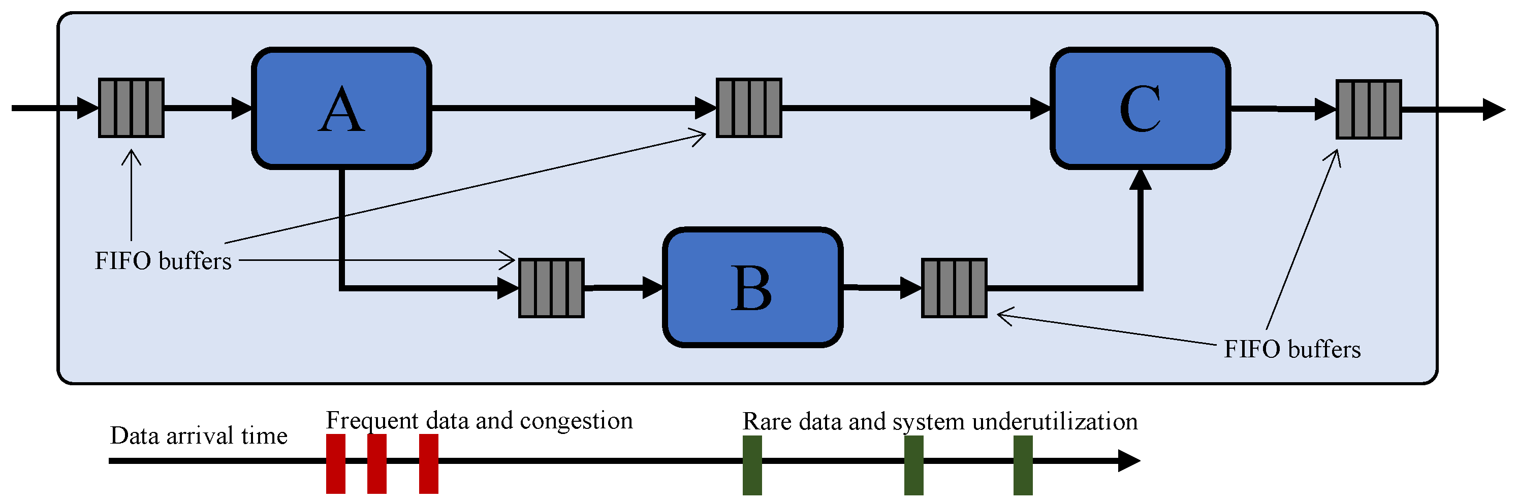
Dataflow architectures are widely used to implement hardware systems that can elaborate a set of incoming data to produce the corresponding results. They are based on a set of concurrent hardware modules that communicate through First-In-First-Out (FIFO) buffers with a producer–consumer paradigm. An example is shown in Figure 1. Such buffers implement a latency-insensitive protocol [5] that guarantees correct computation when the producer is not able to provide enough data (leaving the buffers empty) or when the consumer is not able to consume enough data (leading to data accumulation in the queues). Both these cases can lead to system congestion or poor performance. A traditional solution is to design the accelerator by considering the worst-case scenario, aiming at supporting the fastest input rate. In many cases, it is impossible to optimize the accelerator in this way and the designer needs to use approximated implementations. While approximated solutions are fast and can avoid system congestion for the input buffers, they introduce errors in the output results. Furthermore, since the execution becomes faster than before, the congestion can move to the output buffers. We, thus, need a smarter way to create dynamically tunable accelerators, i.e., architectures that can dynamically change the execution speed (and corresponding error) based on the current workload conditions.

Example 1.

Consider a moving-average filter as a case study. The size of the sampling window can be dynamically adjusted to read more or fewer values, leading to different execution times and errors in the computation of the average. Our goal is to understand how to adjust the window size to achieve a given throughput while minimizing the approximation error. In this case, using the fastest solution for the entire computation leads to achieving the given throughput, but the error is around 90%. An alternative approach uses a threshold control system that determines the best configuration for the accelerator based on the number of elements in the buffers. For example, we can use a system where:

$$\begin{array}{c}\hfill W_1=siz{e}_{buffer}/N_{conf}\\ \hfill W_i=W_1\ast \left(i\right)\end{array}$$

where $siz{e}_{buffer}$ is the size of the input buffer, $N_{conf}$ is the number of available configurations, $W_i$ is the maximum number of elements allowed in the buffer for configuration i (threshold), and i ranges between i and $N_{conf}$. When the buffer number exceeds a threshold, the accelerator is moved to the next (and faster) configuration. This system reduces the error, but it does guarantee that the constraint on the response time is respected. Furthermore, an accelerator can continuously change its configuration when the number of buffer elements fluctuates around one of the thresholds (hysteresis loops).

In this paper, we aim to model the problem as a Markov Decision Process to correctly set the controller’s thresholds while minimizing the approximation error. In queuing theory, an M/D/1 (Markov/Deterministic/1) queue [10] represents a single server queuing process in which the jobs arrive with a Poisson distribution, and the overall service time is deterministic. The jobs are served in their order of arrival (as in FIFOs), and the successive job forms a m-state Markov chain {0, 1, 2, 3,…}, where the value corresponds to the number of entities in the system (the configurations in our case). So, arrivals move the process from position i in the chain to position $i+1$. Queues based on Markov processes may occur in practice when a service adjustment is required (such as the case of inputs arriving at a variable rate). If we count the service time of a job and its time in the system, the different service times correspond to transitions in the Markov chain (i.e., our configuration changes).

3. Related Work

Approximate systems are widely used to reduce the area, power consumption, or latency of a circuit, when the given application can tolerate a certain computational error. Approximate systems are created both at hardware and software levels [7,11]. Hardware approximation can achieve larger benefits, for example, the generation of smaller circuits. On the contrary, software approximation is more flexible and can be tuned more easily based on application requirements.

Software-level approximation trades off accuracy and performance [12,13,14]. Memoization speeds up computation by storing the results of expensive function calls with the same inputs [15]. Skipping some iterations of a loop (loop perforation [12]) or even entire tasks (task skipping [16]) can significantly reduce execution time. Software approximation enables the creation of multiple variants (e.g., alternative codes) that can be dynamically selected based on the workload conditions and the application requirements (multi-versioning [17]). This technique is difficult to directly apply in hardware, since it requires additional resources for each variant.

Customizing data precision is a popular approximation to create smaller components. For example, Gao et al. [18] determined the effects of data-precision manipulation on outputs. Vayerka et al. [19] used genetic programming to create a library of approximate components (e.g., adders and multipliers) to be used in HLS. However, approximating an entire circuit with this method is unfeasible due to its exponential complexity. Lee et al. [20] leveraged an HLS-based method to reduce the circuit latency by eliminating or rescheduling operations (similar to task skipping). Nepal et al. [21] used a greedy approach on the hardware behavioral specification to generate a Pareto-optimal set of alternative approximate implementations. Li et al. [22] presented a comprehensive solution for precision optimization, scheduling, and resource assignment during HLS. Any approximation method requires estimating the error that can be obtained with statistical estimations [23] or with RTL simulations. All these approaches can be used to the create the approximate configurations. However, since such implementations are often structurally similar, datapath merging methods enable the creation of multi-variant hardware components [24,25].

Finally, dynamically changing the “speed” of hardware components to reduce congestion requires online monitors and controllers. For example, Mantovani et al. [6] used a local controller to exploit dynamic voltage and frequency scaling (DVFS) in NoC-based architectures. We use a similar approach to analyze the “congestion” on the communication buffers and determine when the component can change implementation, thus, the approximation level. However, as discussed in Section 2, this threshold-based approach is inefficient, because it can create unnecessary configuration changes.

Table 1. Overview of the main characteristics for the related works.

Systems	Description	Advantages	Disadvantages
Gao et al. [18], 2017	data-precision manipulation	A runtime system. Approximate the minimum necessary. Great energy savings.	Controller at software level.
Vayerka et al. [19], 2016	Genetic programming to create a library of approximate components	Automatic generation of optimized hardware libraries. Work at HLS level.	No runtime support. Static approximation. Unfeasible on entire circuit.
Lee et al. [20], 2017	Rescheduling operations to reduce circuit latency	The transformations are at the HLS level. Much faster than other rescheduling methodologies. Higher energy savings.	No runtime support. Near-optimal result. Not applicable directly in hardware.
Nepal et al. [21], 2014	Greedy approach to generate approximate implementations	Automatically discovers approximate design. Area and power savings. Applicable to generic circuits. Is transparent to the design flow.	No runtime support. Static approximation.
Li et al. [22], 2015	Solution for precision optimization at HLS level	Simple. Provides an ILP formulation for precision optimization.	Not applicable to cases that are both data-intensive and control-intensive. No run time support. Unfeasible on complex systems.
Mantovani et al. [6], 2016	A controller for exploiting dynamic voltage and frequency	Enables pre-silicon tuning and design exploration. Implemented in hardware. Higher power savings.	Creates unnecessary configuration changes due to thresholds. Focuses on power optimization rather performance.

summarizes the advantages and disadvantages of the presented works. We aim at implementing a smarter approach based on queue models, which have been successfully used for runtime resource allocation in multicores [10]. This paper describes how to create the corresponding hardware microarchitecture that efficiently changes the accelerator’s configuration.

4. Hardware Architecture and Model for Online Predictions

We assume a hardware dataflow accelerator similar to the one in Figure 1. The accelerator has input and output FIFO buffers to decouple computation and communication with latency-insensitive protocols [5]. We also assume that each dataflow accelerator supports dynamic tuning, i.e., it has a set of input parameters that can be used to select an approximated configuration. Each accelerator has K configurations ($k=1,2,3...,K$). Each configuration k is characterized by an execution time ${\tau }_k$ and an execution error ${ϵ}_k$. The entire set of configurations can be obtained by combining approximation techniques and design space exploration as discussed in Section 3. Execution time and error are known at design time and can be obtained analytically or with RTL simulation.

4.1. Key Idea and Architecture

We associate a controller to the dataflow accelerator to be dynamically tuned. The controller selects the configuration to be executed and provides the corresponding identifier to the component. In case of dataflow accelerators composed of multiple sub-components that can be individually tuned, the configuration is characterized by a set of parameters to be provided at the same time to each sub-component. The designer needs to identify in advance configurations (i.e., a combination of parameters) that are inefficient (e.g., due to large errors) and exclude them from the list. However, this process is part of the design exploration process that selects the Pareto set configurations. We add logic to delay the selection until the start of the component’s iteration (i.e., when it reads data from the input FIFOs) to avoid inconsistencies during the computation. The approach is valid for both ASIC and FPGA implementations. In case of FPGA implementations, this approach is much faster than partial dynamic reconfiguration, since the hardware is deployed on the configuration logic only once, and it does not require any further changes during execution.

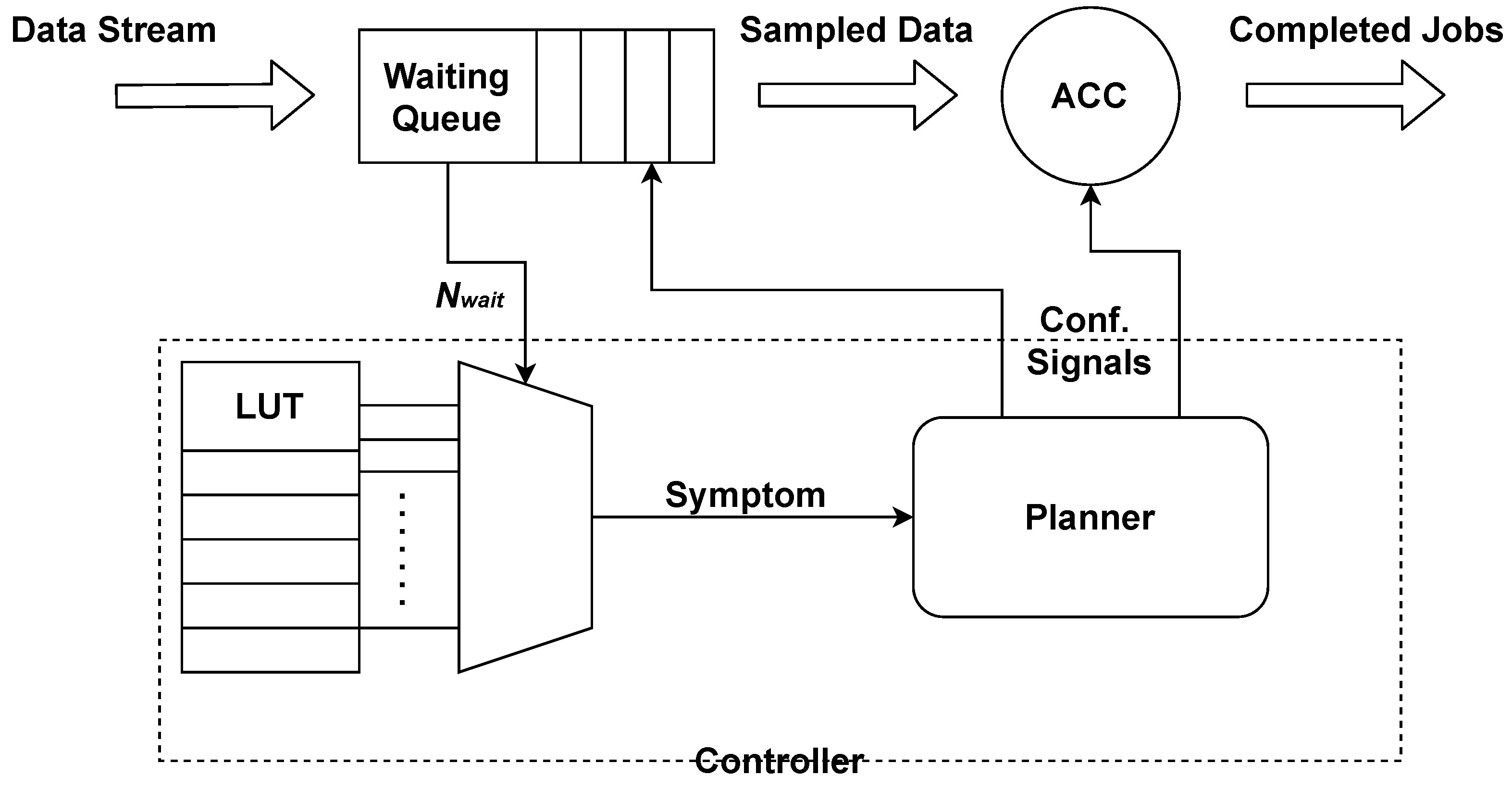
The controller includes the logic to detect congestion and to “speed-up” the computation, and it is parametric with respect to the number of configurations in the Pareto set of the supervised component. To monitor the execution, each controller is connected to the input FIFO buffers with full, almost-full, and empty signals. The status of the input queues is monitored at regular interval (called observation time). When one of the input FIFOs is almost-full, the controller selects a faster configuration for the component to facilitate emptying the queue. Instead, when the input queue becomes empty, the controller can select a more accurate but slower configuration to improve the accuracy. Figure 2 shows an example of the resulting hardware architecture.

The controller does not require specific information on the configurations, because it assumes they are ordered from fastest to slowest (e.g., configuration i is the fastest with no approximation error). This approach is similar to the use of fine-grained DVFS with integrated voltage regulators [6]. The selection of the next configuration requires avoiding hysteresis loops around the buffer thresholds (see Section 2). For this reason, our controller is based on queue models.

4.2. Queue Modeling for Predicting the Response Time

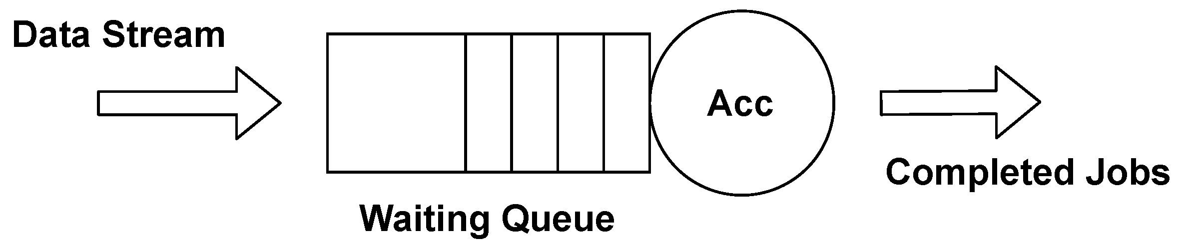
The proposed model aims at providing a suitable runtime policy for configuring the accelerator to minimize the approximation error while meeting a specified constraint on the response time. In this work, we model average response time R using the theory of queuing networks. We model the accelerator as a single resource service station (see Figure 3). The accelerator is the resource that serves the transaction, while its queue is modeled as the waiting line of the station. The service time of the station is modeled as the execution time $t_k$ in each one of the different configurations k, while the expected service rate is calculated as ${\mu }_k=1/{\tau }_k$. Given the balance equation, the job arrival rate $\lambda$ of an application represents the throughput required by the user. It is measured in Job/s, and it depends on the activity to be monitored at runtime.

To enable runtime management, as described previously in the paper, the controller has to maintain and dynamically evaluate the expected average response time. If we consider that the job arrival times can be modeled as a continuous-time Markov process, and, in particular, job interarrival times are exponentially distributed with the mean $\lambda =1$, we can produce a prediction model for R by modeling the problem as an M/D/1 Markov process, i.e., arrivals are determined by a Poisson process (M), job service times are deterministic (D), and there is a single resource service station (1).

In the M/D/1 model, the expected number of jobs in the system (either waiting in queue or being served) in the steady state is given by:

$$\rho ({\mu }_k,\lambda )=\lambda /{\mu }_k$$

(1)

$$N({\mu }_k,\lambda )=\rho ({\mu }_k,\lambda )+{\left[\rho ({\mu }_k,\lambda )\right]}^2/2[1-\rho ({\mu }_k,\lambda )]$$

(2)

where $\rho$ is the system utilization, i.e., the fraction of time in which the system is busy. Given Equations (1) and (2), we can build a prediction model for R by using Little’s law:

$$R({\mu }_k,\lambda )=N({\mu }_k,\lambda )/\lambda$$

(3)

where R only depends on the arrival rate $\lambda$ and the estimated service rate ${\mu }_k$.

We use this model to find the maximum arrival rate that guarantees a response time under a user-defined bound in each configuration. So, from configuration k we derive the estimated ${\lambda }_{max,k}$ that matches a specific amount of jobs (elements) $W_k$ in the waiting queue:

$$W_k={\lambda }_{max,k}\ast ob{s}_{time}$$

(4)

where ${\lambda }_{max,k}$ is predicted from the inverse of Equation (3), and $ob{s}_{time}$ is the observation time of the queue, i.e., the frequency in which the controller samples the status of the queue. $W_k$ represents the maximum number of elements that can be stored in the queue for which the system is able to achieve the response time R by using configuration k. Once the values are computed for each configuration k, we can generate a lightweight logic that changes the accelerator configuration k to $k+1$ when the number of elements detected in the input buffer exceeds the corresponding bound $W_k$ (and vice versa).

5. Generation Methodology for the Online Controller

Our framework requires the user to specify the characteristics of the K individual configurations along with the execution time ${\tau }_k$ for each of them. It also needs the sizes of the input buffers and the required observation time $ob{s}_{time}$ of the controller. Finally, it requires the description of the accelerator configuration ports and the control signals to correctly apply the decisions.

From these data, the framework computes the M/D/1 model, i.e., the values $W_k$ for each configuration. The solution for configuration k is admissible if the corresponding value $W_k$ is smaller than the size of the input buffers. Otherwise, it means that the input buffers cannot store enough values to achieve the response time. If all models can be computed (i.e., all values $W_k$, our generator automatically produces the Verilog description of the corresponding controller as shown in Figure 2. In particular, the input buffers are extended with logic to count the number of elements currently in the queue ($N_{wait}$). The resulting structure is called the smart waiting queue.

At runtime, the controller samples the waiting queue at regular intervals defined by the observation time. It reads the amount of data stored inside the queue and automatically determines the next configuration for the accelerator, given the current configuration and the number of elements in the queue. The values $W_k$ are stored in a lookup table. Assuming the controller is in configuration k, we have three possible cases (represented by the signal symptom in Figure 2:

• $N_{wait}<W_{i-1}$, i.e., the accelerator is emptying the queue, and it can slow down (going to configuration $i-1$ with more precision;
• $N_{wait}>W_i$, i.e., the accelerator is not able to consume the elements in the queue, which are accumulating, and must accelerate (going to configuration $i+1$);
• $W_i<N_{wait}<W_{i-1}$, i.e., the accelerator can stay in the current configuration.

The planner can apply the decision to the control signals of the accelerator right before the next iteration starts (i.e., the next value is read from the input buffers). Since every iteration is independent of the previous ones, this mechanism ensures the correct execution of the acceleration when changing the configurations.

We implemented the generator of the controller in PyVerilog [26]. It receives a json configuration file as input with all necessary information about the target accelerator and extends the original design with the corresponding controller, directly generated in Verilog.

6. Experimental Results

To evaluate our solution, we applied this method to the five accelerators described in

Table 2. Benchmark Characteristics.

Circuit	Description	Application	Input Stimuli	Quality Measure
ave8	Moving Avg Calculator	Signal processing	1000 random integers	MAPE
fir	Finite Impulse Response Filter	Signal processing	1000 random integers	MAPE
sobel	Sobel Edge Detector	Image processing	1920 × 1080 image	PSNR
gs	Grey Scale Filter	Image processing	256 × 256 image	PSNR
gs+sobel	Two accelerators in series	Image processing	256 × 256 image	PSNR

. We used two signal processing benchmarks (DSP) and two image processing benchmarks (IP) [9]. The fifth benchmark was a combination of two other accelerators. We used this example to show how the methodology can be applied to a complex accelerator composed of sub-components. The same table describes also the input stimuli and the quality metric used to evaluate the accuracy of the output results. In this work, we used Mean Average Percentage Error (MAPE) for the DSP applications and Peak Signal-to-Noise Ratio (PSNR) for the image processing ones. We computed MAPE as

$$MAPE=1/N\sum _1^N(G{O}_i-A{O}_i)/G{O}_i$$

(5)

where $G{O}_i$ is the golden output (i.e., the correct/original one), $A{O}_i$ is the output of the approximate description, and N is the total number of inputs. We computed PSNR as

$$PSNR=10\ast log({255}^2/MSE)$$

(6)

where MSE (Mean Square Error) is defined as

$$MSE=\frac{1}{N}\sum _1^N{(G{O}_i-A{O}_i)}^2.$$

(7)

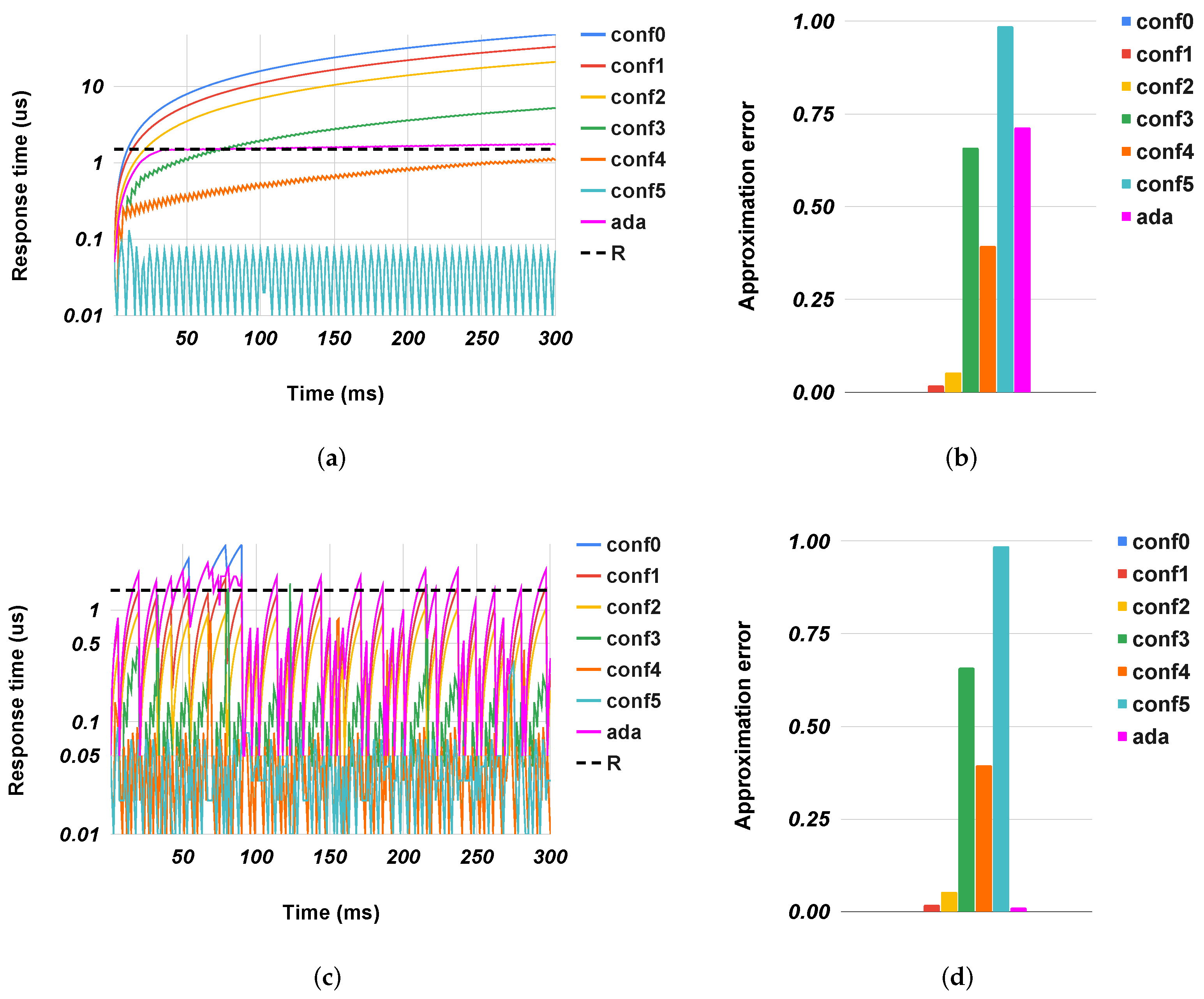
We created six different configurations for each benchmark, where conf0 was the slowest (with no approximation) and conf5 was always much faster than the target response time.

To test the system under dynamic conditions, we created three workload situations, with highly-congested, congested, and uncongested traffic. In our experiments, we set the response time R to $1.5$ us, which was kept constant across all the benchmarks, and an observation time of $1.28$ us, which was the minimum time to fill half of the input buffers. The given response time was set to a value that can be never achieved with conf0 (i.e., the precise configuration), demanding introducing approximations to achieve it.

In our experiments, we evaluated the FPGA implementations, while the ASIC onesweare completely equivalent. For each design, we used Xilinx Isim 2018.3 to evaluate the performance and the approximation error and Xilinx Vivado 2018.3 to target a Xilinx VC707 board (equipped with a Virtex-7 XC7VX485T FPGA) with a target frequency of 100 MHz to evaluate the resource overhead introduced by our controller.

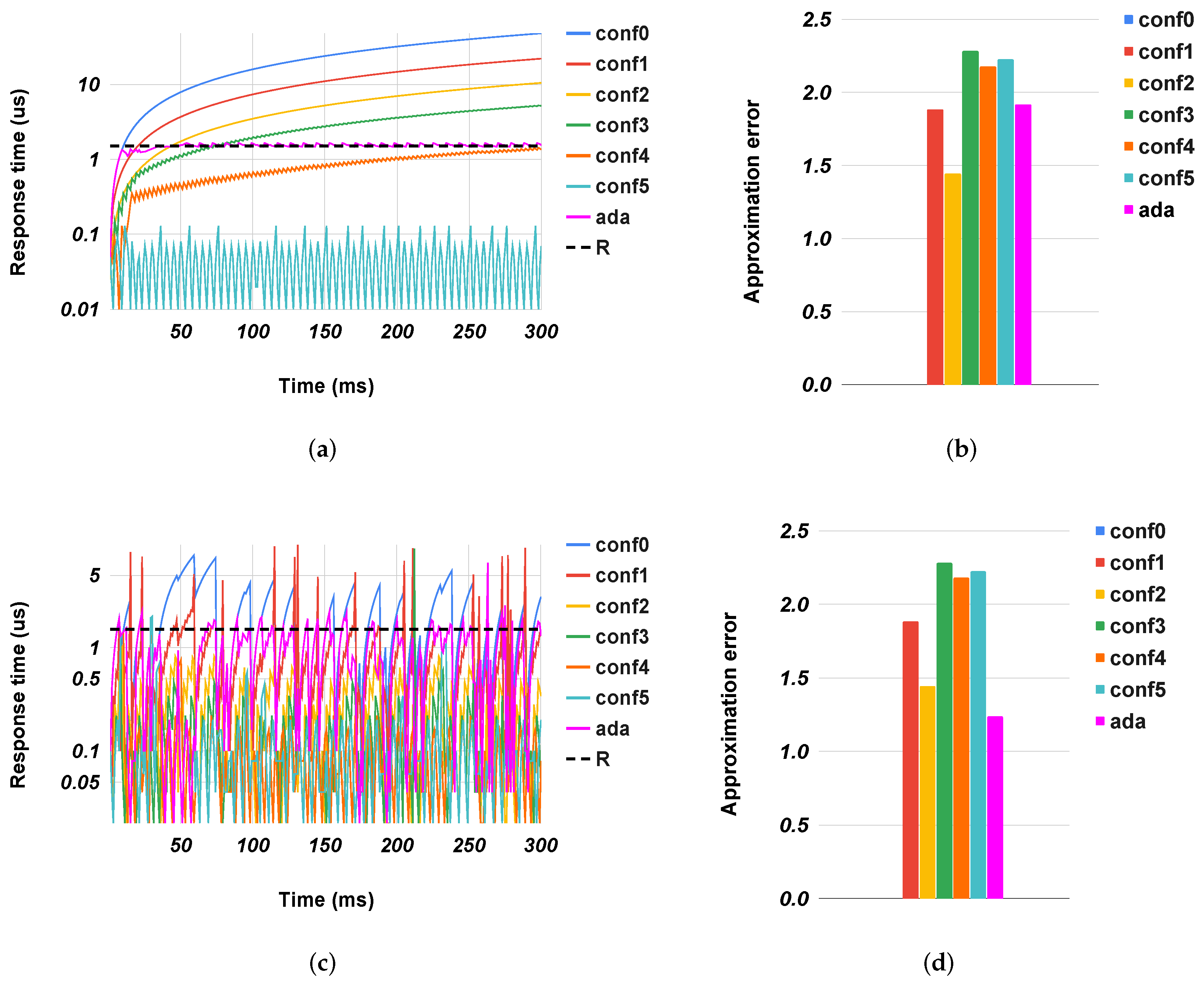
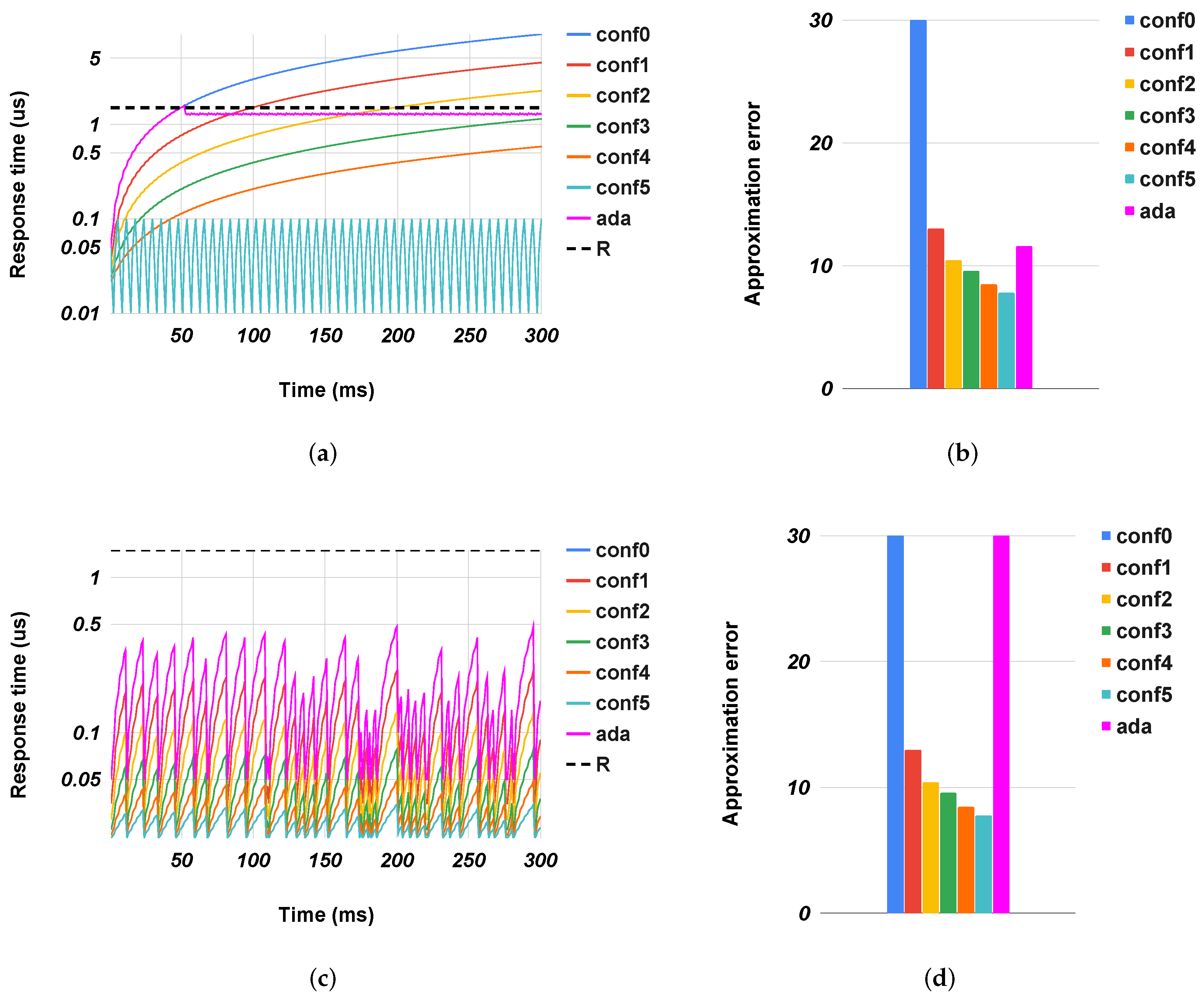
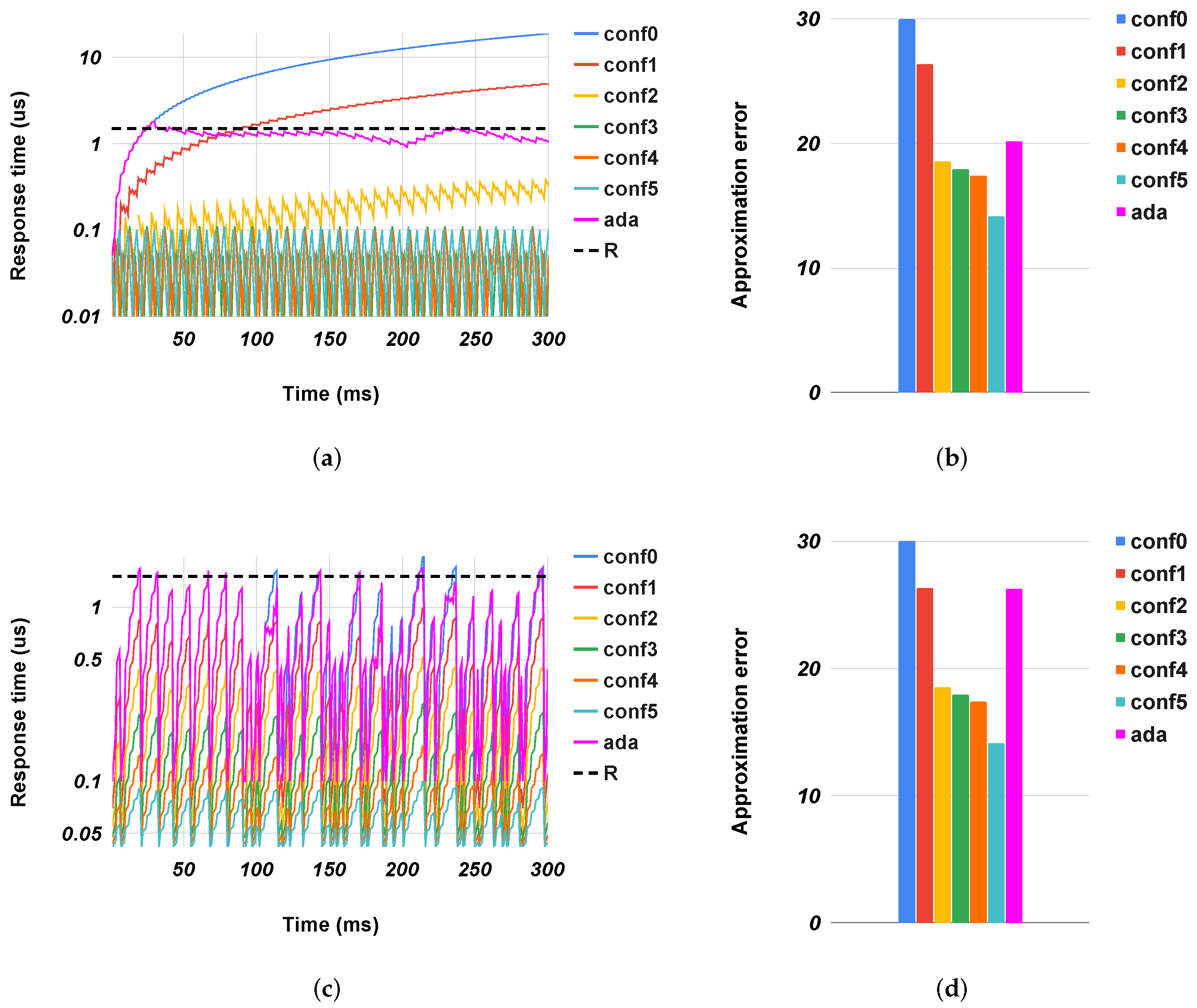
Figure 4, Figure 5, Figure 6, Figure 7 and Figure 8 show the evolution of the response time of the different accelerators over time, along with the quality metrics in the case of preset configurations for the accelerators (from conf0 to conf5) or when they used our method (ada). For clarity, we show only the extreme cases: highly congested and uncongested situations. In congested systems, the response time grew constantly over time to a maximum value. This value was an intrinsic characteristic of the system, and it depended on factors such as the size of the input queue(s), the source of the arrival packets, and the processing speed. Conversely, in uncongested systems, the response time had a trend with peaks. These two behaviors depended exclusively on the inbound traffic. In the former, there was a continuous flow of packets into the system that stopped solely when the queue was saturated. In the latter, the traffic was sporadic and it always allowed the system to empty the queues. The results showed our controllers correctly configured the accelerators to satisfy the response time with a quality metric better or an error less than the ones obtained with fixed configurations. In all cases, the response time was close to the expected one (exploiting the speed of approximate configurations (conf4 and conf5), while limiting the error as configurations conf0 and conf1.

Table 3. DSP Results.

Test	Highly Congested		Congested		Uncongested
	R	MAPE	R	MAPE	R	MAPE
ave8	+30.9%	−27.6%	+148.1%	−92.3%	−1.2%	−40.7%
fir	+16.9%	−16.3%	+6.5%	−21.3%	−36.5%	−33.8%

and

Table 4. IP Results.

Test	Highly Congested		Congested		Uncongested
	R	PSNR	R	PSNR	R	PSNR
sobel	+113.2%	−21.4%	−1.4%	−3.5%	−	−
gs	+10.9%	−12.5%	+9.8%	−30.2%	−3.4%	+0.4%
gs+sobel	+80.3%	−59.8%	+53.2%	−61.1%	+12.8%	−62.8%

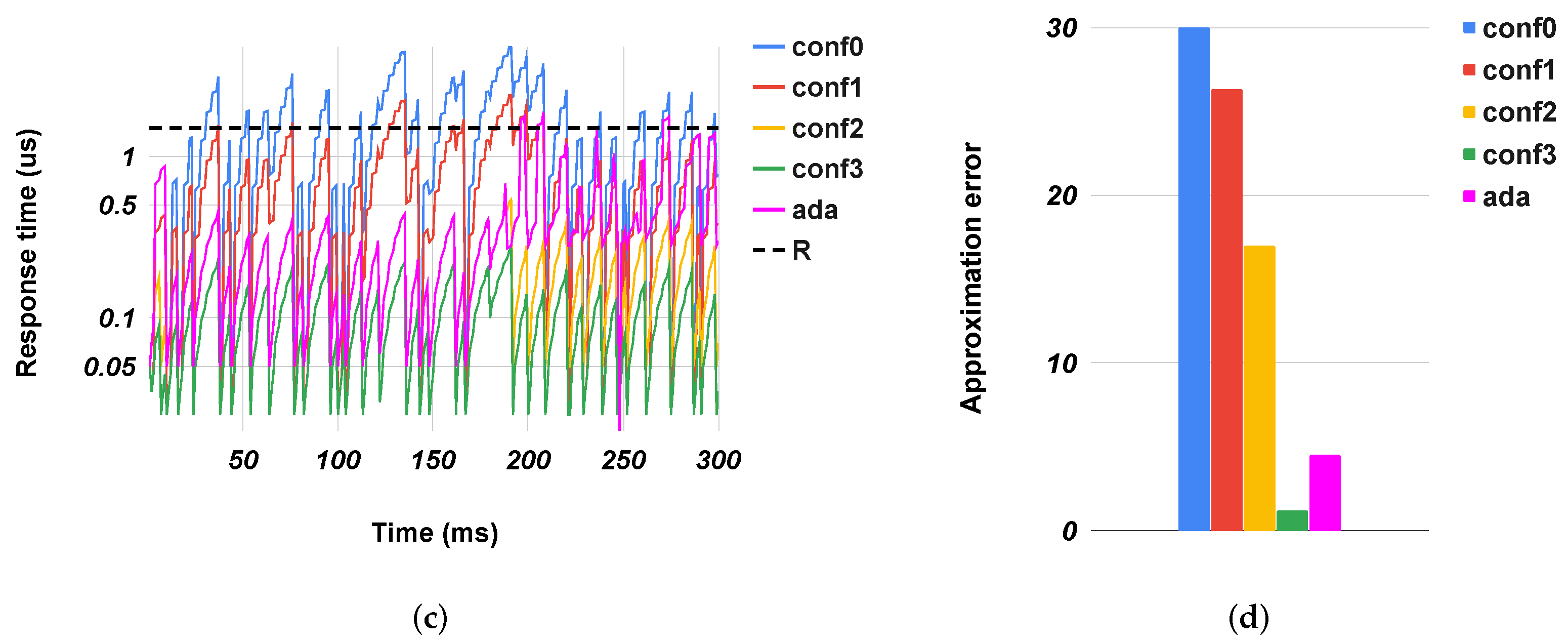
show the corresponding metrics in all three scenarios. The error was always less than the one obtained from the preset configurations except for gs in uncongested cases where the controller unnecessary sped up the execution of the accelerator. This situation happened because, even if the traffic was sporadic, some packet flows re-filled the input queue. In the graph of Figure 7c, we can see where some conf0 peaks exceeded the target response time. The controller interpreted these events by preparing the accelerator for a continuous arrival of packets, but this did not happen. So for a time window that corresponded to the observation time, the system went faster than needed, leading to a slight degradation in the quality of the results. In general, the system adjusted itself based on the workload conditions, trading off accuracy and speed as needed. For example, in the highly-congested scenario (Figure 6a,b), the overall sobel PSNR had a value close to the one obtained with conf1, while only conf4 met the target response time but with much worse PSNR. Conversely, in the uncongested scenario Figure 6c, the system adjusted itself to the most precise configuration (conf0) without any metric degradation.

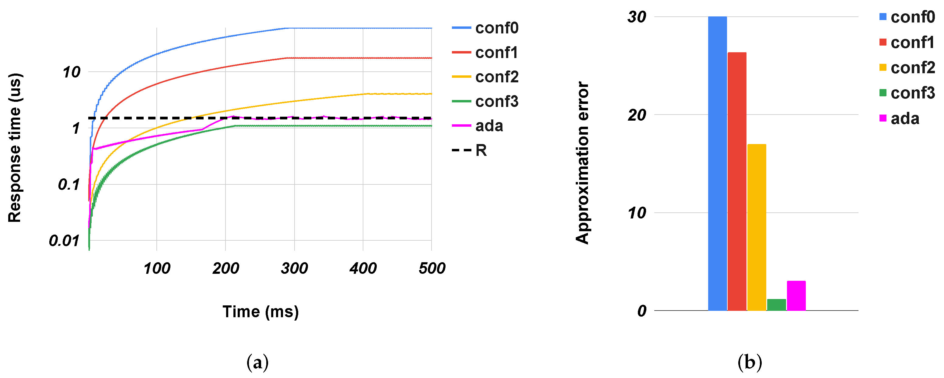
In the gs+sobel, Figure 8, we tested a system with two accelerators in series: gs followed by sobel. This experiment aimed to show how to apply our controller to a multi-module system composed of modules that can be approximated independently. In this benchmark, we used only four configurations, because some of them had $W_i$ larger than the size of the buffers, making them unfeasible. Furthermore, in this case, the controller allowed the accelerator to meet the given response time while improving the final error. Note that the overall PSNR degradation was large due to an intrinsic characteristic of the benchmark rather than a problem in our methodology.

From the synthesis viewpoint,

Table 5. Controller and Smart Logic Area Overhead.

Circuit	Slice LUTs	Slice Registers
ave8	+2.2%	+5.5%
fir	+2.1%	+6.4%
sobel	+3.4%	+8.7%
gs	+0.3%	+0.2%
gs+sobel	+0.3%	+0.2%

shows that the enhanced accelerator took a negligible overhead and, as expected, its impact decreased as the complexity of the target module increased. This overhead was significantly less than the one obtained in previous approaches, because our method was based on a simple lookup table rather than complete state machines, such as in [6].

7. Conclusions and Future Work

We presented a solution to create dataflow accelerators that can dynamically trade off execution latency and quality of results to meet a given response time in case of inputs arriving at an unpredictable rate. We modeled the system as a Markov queuing model to predict the response time and dynamically adjust the speed of the accelerator. Our solution can meet the response time with a final error that is lower than the one obtained by always using the fastest implementation. Our solution also has minimal hardware overhead. In the future, we will work on methods to scale our solution to accelerators composed of multiple modules, considering the case of queues between individual modules, both on the design of the single components and the controller(s), and on upgrading the controller to manage multiple approximation techniques. These extensions contain many challenges, from selecting approximations and studying their impact on the whole system to coordinating multiple controllers to ensure correct execution.