1. Introduction
Online discussions generate a huge amount of data every day, which are hard to process manually by a human. The processing of this discourse content of social networks can bring useful information about the opinions of the crowd on some web trend, political event, person, or product. Approaches to sentiment analysis, particularly to opinion classification, can be used in recognition of antisocial behavior in online discussions, which is a hot topic at present. Negative opinions are often connected with antisocial behavior; for example, “trolling” posting behaviors. This approach can also be used in HRIs (Human–Robot Interactions), where a robot can use information about the polarity of an opinion or mood of the human, in order to communicate appropriately. When a robot communicates with a human (e.g., an elder), it must choose one from many answers which are suitable to the situation. For example, it can choose an answer which can cheer up the person, if it has information that the current emotional situation/mood of the person is sad. It can also adapt its movements and choose a movement from all possible movements, in order to cheer up the human. Therefore, understanding of the emotional moods of humans can lead to better acceptance of communication with robots by humans.
Opinion analysis can be achieved using either a lexicon-based approach or a machine learning approach. These approaches are used, in opinion analysis, to distinguish between positive or negative (sometimes also neutral [
1]) opinions with respect to a certain subject. Machine learning approaches are most often based on the Naive Bayes classifier, Support Vector Machines, Maximum Entropy, k-Nearest Neighbors [
2,
3,
4], or Deep Learning (i.e., based on neural network training) [
5,
6]. The study [
5] presented an approach based on a new deep convolutional neural network which exploits character- to sentence-level information to perform sentiment analysis of short texts. This approach was tested on movie reviews (SSTb, Stanford Sentiment Treebank) and Twitter messages (STS, Stanford Twitter Sentiment). For the SSTb corpus, they achieved 85.7% accuracy in binary positive/negative sentiment classification, while for the STS corpus, they achieved a sentiment prediction accuracy of 86.4%. The study [
6] proved that deep learning approaches have emerged as effective computational models which can discover semantic representations of texts automatically from data without feature engineering. This work presented deep learning approaches as a successful tool for sentiment analysis tasks. They described methods to learn a continuous word representation: the word embedding. As a sentiment lexicon is an important resource for many sentiment analysis systems, the work also presented neural methods to build large-scale sentiment lexicons.
The study [
7] presented an approach for classifying a textual dialogue into four emotion classes: happy, sad, angry, and others. In this work, sentiment analysis is represented by emotional classification. The approach ensembled four different models: bi-directional contextual LSTM (BC-LSTM), categorical Bi-LSTM (CAT-LSTM), binary convolutional Bi-LSTM (BIN-LSTM), and Gated Recurrent Unit (GRU). In this approach, two systems achieved Micro F1 = 0.711 and 0.712. The two systems were merged by assembling, the result of which achieved Micro F1 = 0.7324.
However, machine learning methods have a disadvantage: they require a labelled training data set to learn models for opinion analysis. An interesting fact is that the lexicon approach can be used for the creation of labelled training data for machine learning algorithms.
On the other hand, the lexicon-based approach requires a source of external knowledge, in the form of a labelled lexicon which contains sentiment words with an assigned polarity of opinion expressed in the word. The polarity of opinion has the form of a number that indicates how strong the word is correlated with positive or negative polarity, which is assigned to each word in the lexicon. However, this information is very unbalanced across different languages. In this paper, we focus on adapting and modifying existing approaches to the Slovak language.
This work focuses on an opinion analysis based on a lexicon. In the process of lexicon creation, the lexicon must be labelled to find optimal values for the polarity of words in the lexicon. To assign correct polarity values to words, a human annotator is needed for manual labelling. The manual labelling is time-consuming and expensive. Thus, we tried to replace a human annotator by the Particle Swarm Optimization (PSO) algorithm, as lexicon labelling can be considered an optimization problem. The goal of labelling is to find an optimal set of polarity values; that is, labels for all words in the generated lexicon. These labels are optimized recursively until the opinion classification of texts in data sets using this lexicon with the new labels gives the best results. Therefore, the resulting values of the Macro F1 measure of the opinion classification represent the values of the fitness function in the optimization process. We compare the effectiveness of opinion classification using the lexicon labelled by PSO and using the lexicon annotated by a human.
On the other hand, even when we use the best lexicon, it may still not cover all sentiment words. For this reason, some analyzed posts could not be classified as having positive or negative opinion. To solve this problem, we extend the lexicon approach with a machine learning module, in order to classify unclassified posts using the lexicon-based approach. This module was trained on training data labelled using a lexicon approach for opinion classification. We applied the Naive Bayes classifier to build the module.
The contributions of the paper are as follows:
A new approach to lexicon labelling using the PSO algorithm is presented. PSO optimizes the values of opinion polarity for all words in a labelled lexicon, where the fitness function is represented by the effectiveness measure of sentiment analysis using the labelled lexicon. This automatic labelling avoids the subjectivity of human labelling.
We generated 60 lexicons using PSO (30 small and 30 big lexicons) for an analysis of the distributions of value polarities in lexicons and an analysis of the values preferred by PSO, in comparison with those preferred by a human.
We present a hybrid approach which integrates a machine learning model into the sentiment analysis method, in order to classify texts not containing words in the lexicons.
Extending the new sentiment analysis approach by topic identification in the texts and providing a new means for the interactive combination of switch and shift negation processing.
The creation of two lexicons—Small and Big—in the Slovak language and the creation of a new General data set of short texts. The lexicons (Small and Big, labelled by human) and the General data set are available at (
http://people.tuke.sk/kristina.machova/useful/).
The proposed approach is focused on lexicon-based sentiment analysis. The effectivity of a lexicon approach to sentiment analysis depends on the quality of the used lexicon. The quality of the lexicon is influenced by selection of words in the lexicon, as well as by a measure of precision of the estimated polarity values of words in the lexicon. Our approach uses PSO and BBPSO for the optimal estimation of polarity values. The deep learning method cannot satisfactorily generate the polarity values of words in the lexicon, as clear information about these weight values is lost in the large number of inner layers involved. On the other hand, deep learning can be successfully used in the auxiliary model for the hybrid approach trained by machine learning methods. It is generally assumed that deep learning can achieve better results than the Naive Bayes method in the field of text processing.
2. Related Works
Lexicon-based approaches to opinion analysis require a sentiment lexicon to classify posts as having positive or negative opinion. The lexicon can be generated in three ways: manual, automatic, and semi-automatic. Manually generated lexicons are more accurate and usually involve only single words. They can be translated from another language or collected from a corpus of texts. The value of polarity can then be copied from the original lexicon or calculated from the corpus, based on some metrics. However, this approach is time-consuming. A majority of lexicons separate words into positive and negative groups [
8] or provide additional types of words, such as intensifiers (words that can shift polarity) [
9,
10]. On the other hand, lexicons such as the Warriner lexicon [
11] or the Crowdsourcing, a word–emotion association Lexicon [
12] provide some additional information about the value of polarity for each word. Polarity values allow us to compare the polarities of words and to find more positive and negative words.
Automatically generated lexicons require less human effort. They assign polarity values based on relationships between words in existing lexicons (e.g., SentiWordNet) [
13]. These lexicons contain automatically annotated WordNet synsets, according to their degrees of positivity, negativity, and neutrality. In the WordNet-Affect [
14], emotional values were added to each WordNet synset. SenticNet [
15] includes common-sense knowledge, which provides background information about words. The main weakness of automatically generated lexicons is that they might contain words without polarity or incorrectly assigned polarities. For this reason, the semi-automatic generation of lexicons was introduced. These lexicons are created automatically and are then manually corrected by a human.
Various optimization methods can be used for lexicon labelling. For example, the study [
16] presented a global optimization framework which provides a unified way to combine several human-annotated resources for learning the 10-dimensional sentiment lexicon SentiRuc. By minimizing the error function, an optimal labelling of the lexicon can be found. The work also presented a sentiment disambiguation algorithm, in order to increase the flexibility of this lexicon. The experiments of sentiment disambiguation achieved nice results (Accuracy up to 0.987), but the experiments of sentiment classification based on different lexicons achieved an F1 rate value between 0.383 and 0.726.
Several studies have also used nature-inspired algorithms for text classification. In the study [
17], Particle Swarm Optimization was applied to find the most useful attributes, which were added as an input for a framework based on Conditional Random Field. PSO has also been used to select attributes and combined with Support Vector Machines to classify reviews [
18]. In this paper, PSO is used to generate numbers which represent the polarity values of specific words in the lexicon.
Escalante et al. proposed an approach for increasing the effectiveness of learning term-weighting schemes using a genetic program [
19]. The schemes were used to improve classification performance. Standard term-weighting schemes were combined with the new term-weighting schemes, which were more discriminative due to the use of the genetic algorithm. They reported an experimental study comprising a data set for thematic and non-thematic text classification, as well as for image classification. Unlike their approach, we use a genetic program to find not only the weights of words, but values of their opinion polarity as well, which is a different problem and cannot be computed only based on the frequency of words in the text. Nevertheless, the average result of their best-performing approaches for all data sets was F1 = 0.775. Our average result for all data sets was Macro F1 = 0.759, which is comparable with the results in [
19].
The study [
20] proposed an approach to simultaneously train a vanilla sentiment classifier and adapt word polarities to the target domain. The adaptation was based on tracking wrongly predicted sentences and using them for supervision. On the other hand, our approach builds a domain-independent lexicon of labelled words. In this paper, the best results of testing on the Movie data set was Accuracy = 0.779. Our best results on the Movie data set (MacroF1 = 0.743, see Table 11) were comparable with the results in [
20]. It is easier to achieve higher results in Accuracy than in F1 rate, even though both measures of classification effectiveness consider both false positive and false negative classifications.
2.1. Nature-Inspired Optimization
Nature-inspired algorithms are motivated by biological systems such as beehives, anthills, and swarms of fish, birds, and so on. They investigate the behaviors of individuals in a population, their mutual interactions, and their interactions with an environment. For example, PSO was inspired by a flock of birds searching for food. We suppose that only some birds know about food and where it is situated. Therefore, the best strategy is to follow the individual nearest to the food. Every individual in a population represents a bird and has a fitness value in the search space.
Particle Swarm Optimization is an optimization algorithm which is inspired by a flock of birds. PSO converges to the final solution; in this case, it has the form of the best-labelled lexicon. The possible solutions are called particles, which are parts of the population. Each particle keeps its best solution (evaluated by the fitness function) called
pbest, while the best value chosen from the whole swarm is called
gbest. The standard PSO consists of two steps: change velocity and update positions. In the first step, each particle changes its velocity towards its
pbest and
gbest [
21]. In the second step, the particle updates its position. A new position is calculated, based on previous position and a new velocity. Each particle is represented as a vector in a D-dimensional space. The i
th particle can be represented as
Xi = (
xi1,
xi2,…,
xiD). The velocity of the i
th particle is represented as
Vi = (
vi1,
vi2,…,
viD) and the best previous position of the particle is represented as
Pi = (
pi1,
pi2,…,
piD). The best particle in the swarm is represented by
g and
w is the inertia weight, which balances the exploration and exploitation abilities of the particles. The velocity and position are updated using Equations (1) and (2):
where
d = 1, 2, …, D (in our system, D represents the number of words in the dictionary);
i = 1, 2, …, N, where N is the number of particles in the swarm;
n = 1, 2, …, max denotes the iteration number;
r1 and r2 are uniformly distributed random values which avoid the particles falling into local optima; and
c1 and
c2 are important parameters, known as the self-confidence factor and the swarm confidence factor, respectively. They define the type of trajectory the particle travels on, so they control the searching behavior of the particle [
22].
The stopping criteria of the algorithm often depends on the type of the problem. In practice, PSO is run until a fixed number of function evaluations is carried out or an error bound is reached.
PSO uses
pbest and
gbest to update the position of a particle. The impacts of these values were studied in [
23]. In this work,
pbest and
gbest were set as constants and the trajectories of the particles were investigated. These results show that the trajectory can be determined by the difference between
pbest and
gbest. These positions can determine the particle’s movement. Based on this knowledge, a new PSO method was designed; the so-called Bare-bones PSO (BBPSO). BBPSO uses a Gaussian distribution
N(µ,σ) with the mean µ and standard deviation
, as shown in Equation (3):
where µ is the center of
pbest and
gbest, and σ is the absolute difference between
pbest and
gbest. The rand() function is used to speed up convergence by retaining the previous best position,
pbest.
2.2. Naive Bayes Learning Method
Naive Bayes is a probabilistic classifier based on Bayes’ theorem and the independence assumption between attributes.
For n observations or attributes (respectively, words)
x1, …,
xn, the conditional probability for any class
yj can be expressed as Equation (4):
This model is called the Naive Bayes classifier. Naive Bayes is often applied as a baseline for text classification [
2]. We used the Naïve Bayes learning method in two ways:
For the labelling of words in a lexicon.
For learning a model for opinion classification of posts when the lexicon approach fails. This approach to opinion classification is called the hybrid approach and is discussed below.
When we used Naive Bayes for labelling words in a lexicon, all labelled words in the lexicon played the role of attributes in the Bayes learning method. We had to calculate the numerical value representing the measure of polarity of each word in the lexicon. This value is based on probability of the word to belong to a class (positive or negative). We needed a training data set to calculate these values (probabilities). A training data set was used to calculate the probability
P that a word
w from the post text relates to each class
c (positive or negative). Labels assigned using this probability were used to build a lexicon. The probability can be calculated by the simple probability method described by Equation (5):
where
P(wc)—the probability that the word (from class c) is the polarity value of the word.
∑wc—the number of occurrences of word w in class c.
∑w—the number of occurrences of word w in the whole data set.
In case that the word is not assigned to a specific class, the probability would be zero; therefore, a method which returns a very low number, instead of zero, was implemented.
3. Lexicon Generation
There are many approaches for the generation of a lexicon. A lexicon can be generated for a given domain. This lexicon is obviously very precise in this domain, but usually has a weak performance in different domains. Another way is to generate a general lexicon. This lexicon usually has the same effectiveness in all domains, which is mostly not very high.
We generated two lexicons to analyze opinion in Slovak posts using a lexicon approach. We used two different methods of generation: translation and composition from many relevant lexicons. The first (Big) lexicon was translated from English and then extended by a human. It was enlarged by domain-dependent words, in order to increase its effectiveness. The domain-dependent words were words which may be common, but which have different meanings in different domains. For example, the word “long” has a different opinion polarity in the electrical domain (i.e., “long battery life”) than in the movie domain (i.e., “too long movie”). Thus, the Big lexicon was domain-dependent, which is its disadvantage. For this reason, we decided to generate another new (Small) lexicon. This lexicon was expected to be domain-independent, as it was extracted from six English lexicons in which only domain-independent words were included. Domain-independent words are words which have the same meaning in different domains. They were analyzed and only overlapping words from all lexicons were picked up. The advantage of the Small lexicon is its smaller size, in comparison with the Big lexicon. This is an important feature, as each particle in our PSO implementation represents the whole labelled lexicon; more precisely, a set of polarity values for all words in the lexicon. A smaller lexicon, thus, means that a smaller set of labels must be optimized. So, the size of the lexicon influences the time needed to find the optimal solution. The words in the lexicon were selected once, but the labels of those words (i.e., polarity values) were found by optimization using PSO and BBPSO in 60 iterations. During optimization, the labels of the words were recursively changed many times, until the fitness function gave satisfactory results.
For both lexicons, three versions were generated: The first version was labelled manually by a human annotator, the second version was labelled by PSO, and the third one using BBSPO. Then, all versions were used for opinion analysis of post texts in the Slovak language and tested. We could engage more annotators in the process of human labelling, but the subjectivity of labels would remain, and averaging the values of labels may obscure the accurate estimation of the word polarities by one expert human.
The Big lexicon was generated by manual human translation from an original English lexicon [
10], which consists of 6789 words including 13 negations. The generated lexicon in Slovak was smaller than original lexicon, as some words have in Slovak less synonyms than in English. We translated only positive and negative words to Slovak. Synonyms and antonyms of original words were found in a Slovak thesaurus. The thesaurus was also used to determine intensifiers and negations. The final Big lexicon consisted of 1430 words: 598 positive words, 772 negative words, 41 intensifiers, and 19 negations. The first version of this lexicon was labelled by a human. The range of polarity from −3 (the most negative word) to +3 (the most positive word) was chosen to assign the polarity value to each word. For each word in the lexicon, the English form was searched in a double translation. “Double translation” means that each word from the lexicon was translated into English and then was translated back to Slovak, in the case that the word had the same meaning before and after translation, the final form of the word was added to the lexicon.
The Small
lexicon was derived from six different English lexicons, as used in the works [
10,
15,
24,
25,
26,
27]. The English lexicons were analyzed and only overlapping words were chosen to form the new lexicon. To translate these words to Slovak, the English translations from the Big lexicon were used. Overlapping words were found, and their Slovak forms were added to the lexicon. This new lexicon contained 220 words, including 85 positive words and 135 negative words. Intensifiers and negations were not added, as they were not included in all original lexicons. The first version of the lexicon was labelled manually, with a range of polarity from −3 to 3. The details of the lexicons used for the creation of the Small lexicon are as follows:
Hu and Liu lexicon [
10] (4783 positives, 2006 negatives, and 13 opposites)
SenticNet 4.0 [
15] (27,405 positives and 22,595 negatives)
Sentiment140 [
24] (38,312 positives and 24,156 negatives)
AFINN [
25] (878 positives and 1598 negatives)
Taboada lexicon [
26] (2535 positives, 4039 negatives, and 219 intensifiers)
SentiStrength [
27] (399 positives, 524 negatives, 28 intensifiers, and 17 opposites).
4. Lexicon Labelling Using Particle Swarm Optimization
Particle Swarm Optimization (PSO) was chosen as a method for the lexicon labelling, as labelling is an optimization problem where a combination of values of labels for all words in a lexicon has to create the best overall evaluation of the polarity of a given text. PSO is an efficient and robust optimization method, which has been successfully applied to solve various optimization problems. In the optimization process of lexicon labelling using PSO, each particle represents one version of the lexicon for labelling. A lexicon can be encoded as a vector Xi = (xi1, xi2,…, xiD). Each word of the lexicon is labelled by a number, representing the measure of polarity from negative to positive xij ∈ {−3,3}, i = 1, 2, …, N, where N is the number of particles and j = 1,2,…,D, where D denotes the number of words in the lexicon. Thus, the particle size depends on the size of the lexicon.
From the Big lexicon, only positive and negative words were used. Therefore, the particle size was decreased from 1470 to 1370 polarity values. The particle representing the Small lexicon had 220 polarity values. The designed approach is described in the following Algorithm 1:
| Algorithm 1: PSO algorithm |
| generate the initial population |
| for number of iterations do |
| for particle_i do |
| ϕi evaluate particle_i using fitness function |
| ζi compute value of fitness function for pbest of particle_i |
| if ϕi > ζi then update pbest |
| end if |
| if pbest > gbest then update gbest |
| end if |
| end for |
| for each particle_i do |
| for each dimension d do |
| compute new velocity according (1) |
| compute new position according (2) |
| end for |
| end for |
| end for |
| return the value of gbest particle |
The goal of labelling a lexicon using PSO is to find an optimal set of polarity values for all words in this lexicon. One position of the particle represents one potential solution (one set of labels of words), which is recursively changed during the process of optimization. Each potential solution can be represented as a vector in D-dimensional space, where D is the number of words in the lexicon. In our approach, the initial population was generated randomly and then, the PSO method was applied. In PSO optimization, each particle was evaluated based on the fitness function (values of MacroF1). For each actual particle, pbest (particle best) was set and gbest for the whole swarm (global best) was searched. For the next iteration, a velocity of each particle was calculated (1) based on its pbest and gbest, and then the position of the particle was updated using Formula (2). Then, the particle was evaluated again and pbest and gbest were updated again. This process was run recursively until a fixed number of iterations was met. For experiments with standard PSO, the following parameters were used:
inertia weight = 0.729844
number of particles = 15,000
number of iterations = 100
c1 = 1.49618
c2 = 1.49618
max velocity = 2
4.1. Labelling by Bare-Bones Particle Swarm Optimization
Bare-Bones PSO uses a different approach to find an optimal polarity value for each word in a lexicon. BBPSO works with a mean and standard deviation of a Gaussian distribution. The mean and deviation are calculated from pbest and gbest. The process of labelling is shown in the following Algorithm 2:
| Algorithm 2: BBPSO algorithm |
| generate the initial population |
| for number of iterations do |
| for particle_i do |
| ϕi evaluate particle_i using fitness function |
| ζi compute value of fitness function for pbest of particle_i |
| if ϕi > ζi then update pbest |
| end if |
| if pbest > gbest then update gbest |
| end if |
| end for |
| for each particle_i do |
| for each dimension d do |
| compute new position using Gaussian distribution |
| end for |
| end for |
| end for |
| return the value of gbest particle |
BBPSO uses a Gaussian distribution
N(
µid,
σid) with mean
µid and standard deviation
σid. These values are calculated using Equations (6) and (7):
where
d = 1, 2, …, D, with D representing the number of words in the lexicon, and
i = 1, 2, …, N, where N is the number of particles in the swarm.
4.2. Fitness Function for Optimization
The fitness function was based on the lexicon approach used to classify the opinion of post texts in data sets. This classification was provided repetitively with all lexicons generated by PSO (or BBPSO). Every opinion classification using all particular lexicons was evaluated by the F1 rate, which is a harmonic mean between Precision and Recall, calculated by Equation (8). The F1 rate played the role of the fitness function.
The opinion classification was implemented in the following way: Each input post text was tokenized. Each word was compared with words in the temporary test lexicon. If the word was found in the dictionary, the polarity value of the post was updated. If the word was positive, the polarity of the post was increased and if the word was negative, the post polarity was decreased, according to Equation (9):
where
Precision and Recall were calculated based on the comparison of the automatically assigned labels with the gold-standard class labels. These were applied to calculate the F1 rate. However, the final values of the fitness function were not derived from F1 rate, but instead from the MacroF1 rate (10), which better evaluates the performance on an unbalanced data set. The MacroF1 rate (10) shows the effectiveness in each class, independent of the size of the class:
where
The use of this fitness function was based on the defined measure of classification effectivity (MacroF1). All words in the lexicon were repeatedly labelled and the effectivity of opinion classification of texts from the data set using this lexicon (with new labels) was evaluated, until the labels were found to be optimal. In this way, the labelled polarity of words in the lexicon could be domain-dependent, if the data set of texts was domain-dependent. Therefore, we used two data sets: one being domain-dependent (Movie), while the other was domain-independent (Slovak-General). The labelling of a lexicon is an optimization problem and, in this case, supervised learning was used only for computing the values of the fitness function. However, supervised learning was also used for model training in the hybrid approach for opinion classification (see
Section 7.2). This model was then used for classification of texts with a difficult dictionary.
5. Experiments with Various Labelling
5.1. Data Sets
Experiments with different labelling methods were tested on two data sets. The General data set contained 4720 reviews from different websites in the Slovak language. It consisted of 2455 positive and 2265 negative comments. Neutral comments were removed. The reviews referred to different domains such as electronics reviews, books reviews, movie reviews, and politics. The data set included 155,522 words. The Slovak-General data set is available at (
http://people.tuke.sk/kristina.machova/useful/).
The Movie data set [
2] contained 1000 positive and 1000 negative posts collected from rottentomatos.com. The data set was pre-processed and translated to Slovak. All data sets were labelled as positive or negative by human annotators. Each data set was randomly split with a ratio of 90:10—90% for training and 10% unseen posts for validation. All results were obtained on the testing set. The same subsets were applied in all experiments, including the human-labelled lexicon.
5.2. Experiments with PSO and BBPSO Labelling
In the process of optimizing the labelling of the Big and Small lexicons, the initial labelling, a set of polarity values for all words in the lexicon was first found (1370 values for Big and 220 values for Small lexicon; the Big lexicon originally had 1430 words, but only positive and negative words were included in the experiments). This set of values (1370 or 220) represented one particle for PSO optimization. Then, this set of values was changed with the aid of pbest and gbest, until the effectiveness of using the particle (set of labelling values for each word in the lexicon) in the lexicon-based opinion classification was the highest. Within the labelling optimization, not only one but 30 labels for the Small lexicon and 30 labels for the Big lexicon were generated, in order to achieve statistically significant results.
A set of experiments were carried out, where both data sets (General and Movie) were used for testing of labelling for both lexicons (Big and Small). Two methods for labelling these lexicons were tested: using PSO and BBPSO.
Each experiment was repeated 30 times, in order to achieve statistically significant results. The following tables show only the results for the best experiment and the average results of all 30 repeats. The achieved results of these experiments were obtained on the respective validation sets. The results are presented in
Table 1,
Table 2,
Table 3,
Table 4,
Table 5,
Table 6,
Table 7 and
Table 8. The results of these experiments are measured by Precision in the positive class (Precision Pos.), Precision in the negative class (Precision Neg.), Recall in the positive class (Recall Pos.), Recall in the negative class (Recall Neg.), F1 Positive, F1 Negative, and Macro F1.
Table 1 and
Table 2 represent experiments on the Movie data set using the Big lexicon.
Table 1 shows that using the lexicon labelled by BBPSO was more precise for opinion classification than PSO in all cases, with only one exception. Another observation was that, in all experiments, Precision in classification of positive posts was better than Precision in classification of negative posts; however, for Recall, the observation was opposite. The Macro F1 rate in
Table 2 gives us more results. There were no significant differences between classification of positive and negative posts. The important result is that labelling by BBPSO led to a more precise lexicon than labelling by PSO.
Table 3 and
Table 4 represent experiments on the Movie data set using the Small lexicon. Comparison of
Table 1 with
Table 3 and
Table 2 with
Table 4 shows that using the Small and Big lexicons gave very similar results, in terms of Precision, Recall, and Macro F1 rate, on the Movie data set.
We also provide results for four similar experiments on the General data set, which are presented in
Table 5,
Table 6,
Table 7 and
Table 8. The results in
Table 5 show that experiments on the General data set led to similar results to the experiments on the Movie data set. Precision in classification of positive posts was better than classification of negative posts; however, the observation was opposite in Recall.
The results in
Table 5 and
Table 6 show that using the lexicon labelled by BBPSO was more precise for opinion classification than PSO, in most cases.
Table 7 demonstrates that using the Small lexicon on the General data set led to very poor results; only Recall in positive posts gave good results.
The Macro F1 rate, presented in
Table 8, confirms this finding. The reason for this failure could be that the Small lexicon was generated from six English lexicons and only overlapping words from all lexicons were chosen. So, the Small lexicon may have not contained specific words which were important for polarity identification in a given text; that is, it did not contain all necessary words with sentiment polarities needed for the successful sentiment classification of general texts.
The significance test is also provided. Paired sample
t-test was used to prove the statistically significant improvement between PSO and BBPSO. A 95% confidence interval and 29 degrees of freedom were applied. We tested the Macro F1 measure, and the results (see
Table 9) showed that BBPSO was significantly better than PSO.
The
p-value represents the probability that there is no statistically significant difference between the results. The
p-values were small in all cases. This means that the probability that there was no statistically significant difference between the results presented in
Table 1,
Table 2,
Table 3,
Table 4,
Table 5,
Table 6,
Table 7 and
Table 8 is small. Thus, we can say that the difference between the results was statistically significant. This statement is valid with 95% confidence.
The complexity of the automatic labelling of lexicons using the optimization methods PSO and BBPSO is , where is the maximum number of iterations, N is the total number of words in the training set, and D is the number of words in the lexicon. This means that the complexity is linear in the size of the training set and the lexicon. In our case, the General data set contained 155,522 words and the Big lexicon contained 1370 words. The complexity of the lexicon approach for opinion classification, which was used for computing the values of the fitness function, was linear in the size of posts in the training set M and the number of words in the lexicon D, such that its complexity is .
5.3. Comparison of PSO and BBPSO Labelling with Human Labelling
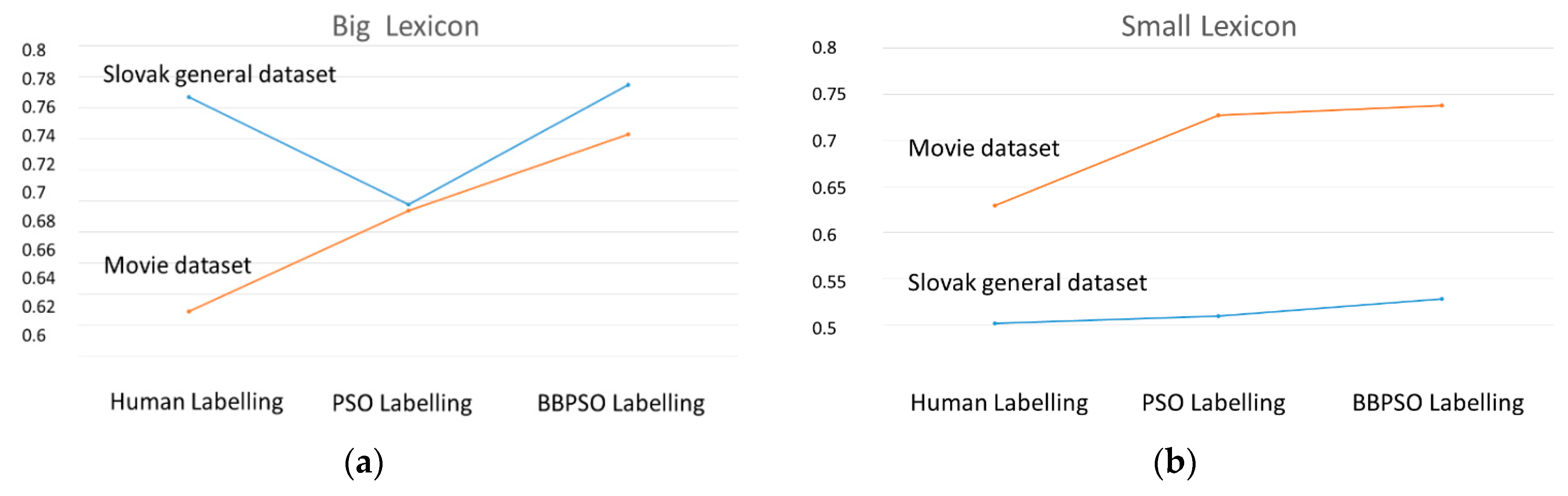
In the previous section, it was shown that BBPSO was better than simple PSO. We wanted to also compare this approach to human labelling. Within this experiment, we decided to evaluate results of the opinion classification only in terms of Macro F1 rate. The results are illustrated in
Table 10. It was shown that automatic labelling using nature-inspired optimization algorithms, especially BBPSO, was better than human labelling of lexicons for the lexicon approach to opinion classification.
The results in
Table 10 confirm the findings in
Table 7 and
Table 8: that using the Small lexicon on the General (Slovak) data set led to very poor results, not only when using PSO and BBPSO labelling but also for human labelling. The most important fact is that BBPSO was able to find the best polarity values for the words in the lexicon, independently of the used lexicon (Big or Small) and data set (Movie or General—Slovak). These results are illustrated also in
Figure 1a,b for the Big and Small lexicons, respectively.
We found seven other approaches which used the Movie data set.
Table 11 contains a comparison of our approach to those other related works with experiments on the Movie data set. For our needs, the data set was automatically translated into Slovak language, which had an impact on the overall results of our tests. The last row of the
Table 11 contains results of our hybrid approach (
Section 7.2) on Movie data set, but the results of the same approach on General dataset were better (Accuracy = 0.865).
6. Distribution of Values of Polarities in Generated Lexicons
The main purpose of this section is the comparison of human labelling and automatic labelling, in order to answer the following questions: Which integer labels are preferred in PSO and BBPSO labelling, in comparison with human labelling? Can the subjectivity of human labelling cause a decrease of effectiveness of lexicon-based opinion classification?
We worked under the assumption that automatic labelling is not subjective, like human labelling. This is because, in the process of PSO labelling, the effectivity of lexicon use in lexicon-based opinion classification is a decisive factor. Many human annotators can easily agree on whether an opinion is positive or negative, but when determining the intensity degrees of the polarity of opinions, it is difficult to reach an agreement. So, labelling using PSO optimization seemed to be a good solution. This assumption was supported by our results, which are shown in
Figure 2,
Figure 3,
Figure 4 and
Figure 5.
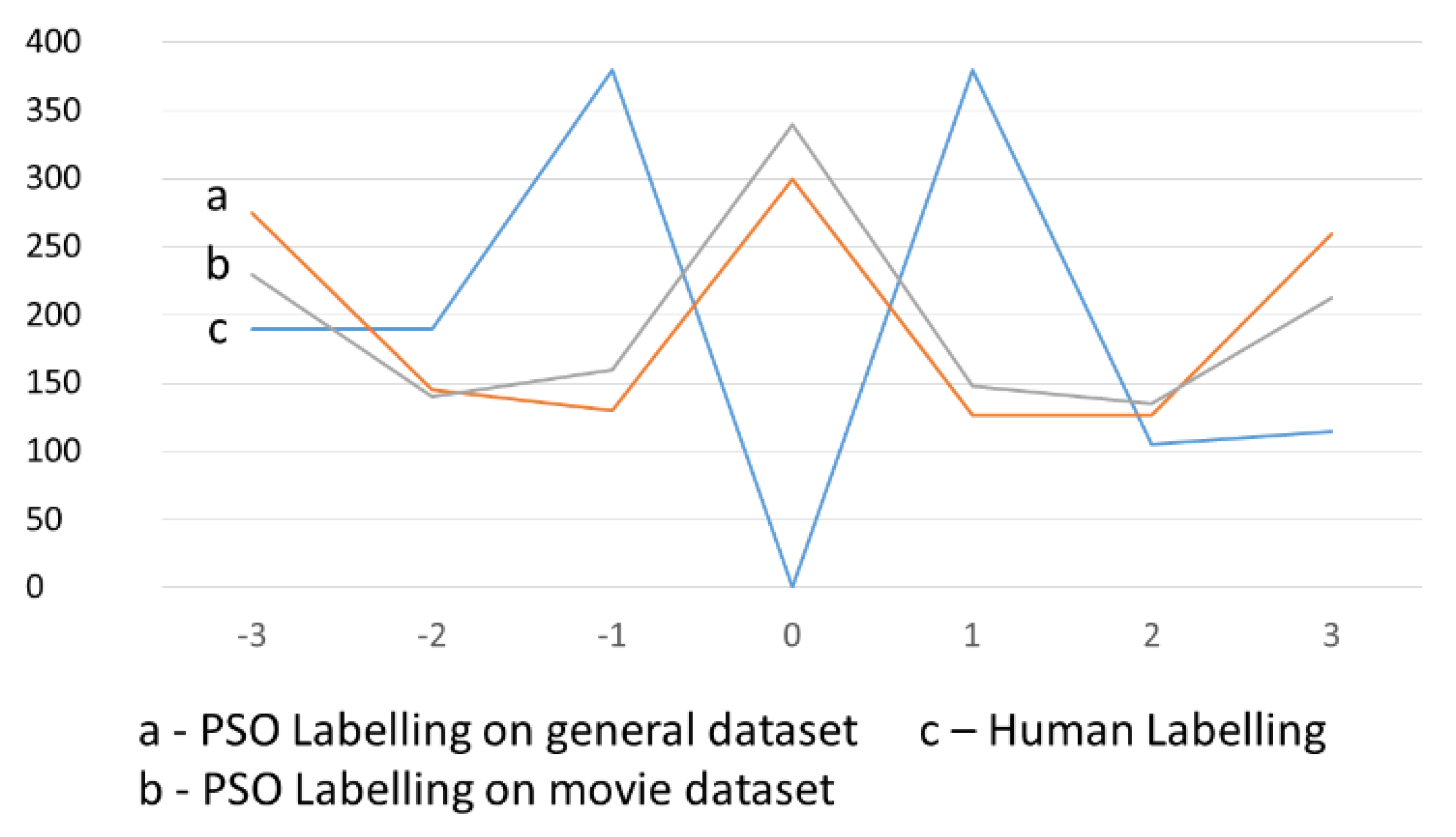
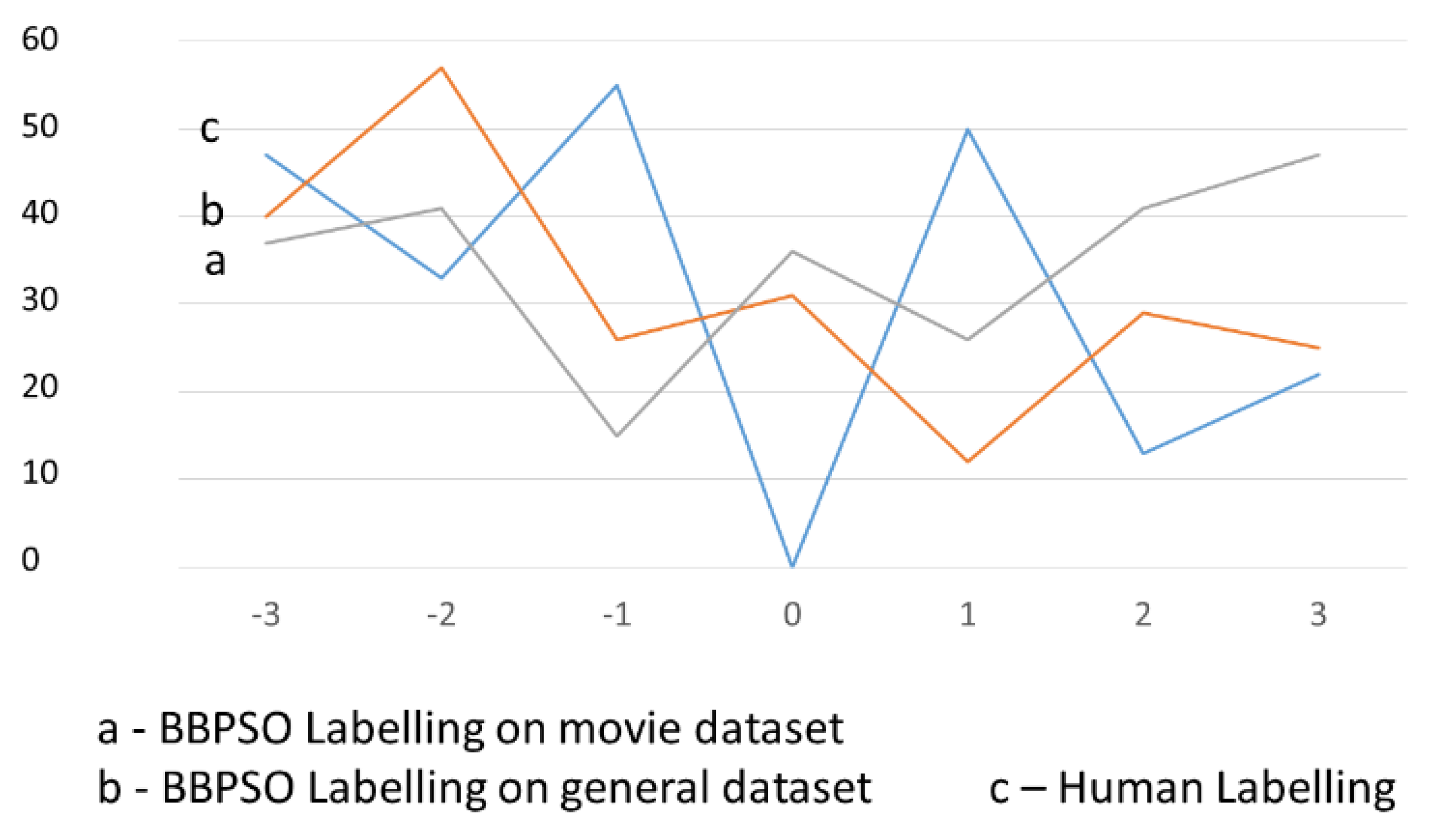
We also examined the distribution of polarity values, which were assigned by the automatic labelling in the interval of integers <−3, +3> in labelled lexicons. We wanted to know if there were some differences between labelling by human and automatic labelling (PSO, BBPSO); in other words, we wanted to find some integer values in the interval <−3, +3> which are preferred by a human or an automatic annotator, respectively. Our findings are illustrated in
Figure 2,
Figure 3,
Figure 4 and
Figure 5.
The models of PSO and BBPSO labelling were generated using both General and Movie data sets. Of course, human labelling is independent of any data set. In
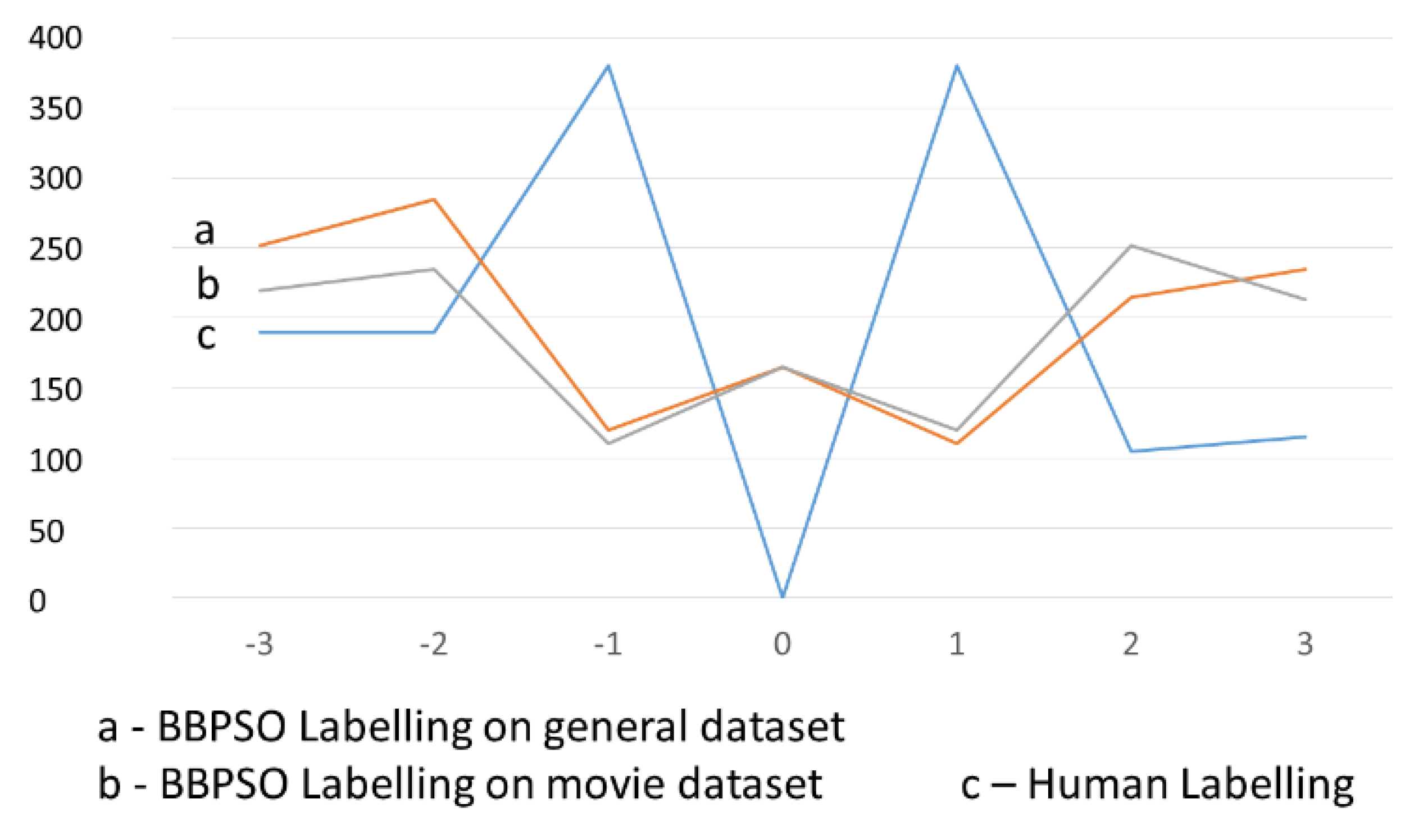
Figure 2 and
Figure 3, the result distributions of the intensity of polarity values in the Big lexicon are shown.
Figure 2 illustrates the results of comparison of PSO and human labelling, while
Figure 3 illustrates the comparison of BBPSO and human labelling. We can see, in these two figures, that the human annotator avoided labelling words with zero. They expected only positive or negative words in the lexicon and no neutral ones. On the other hand, PSO frequently used a zero-polarity label. BBPSO also used zero polarity values, but they were not applied as often.
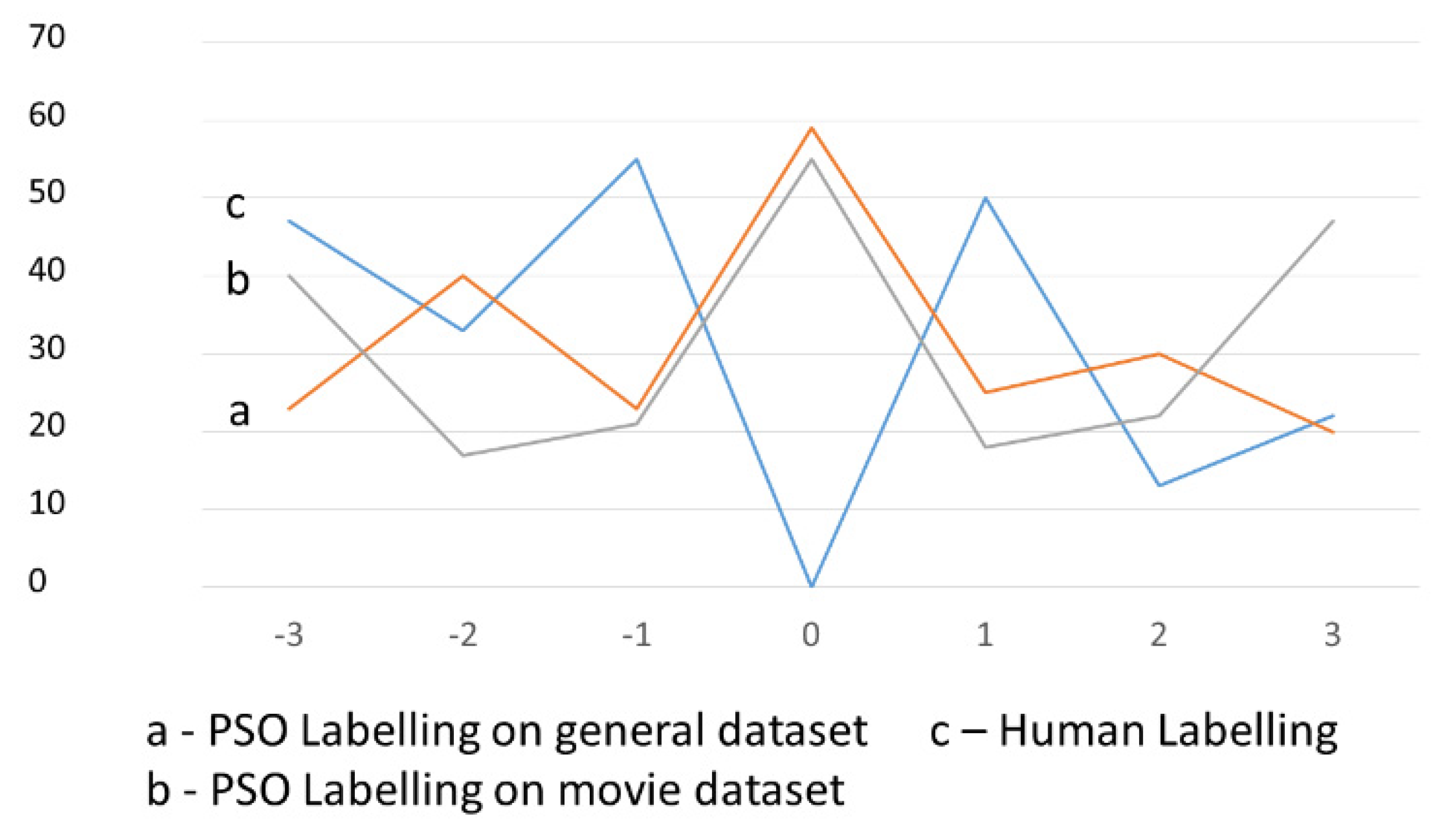
We ran similar experiments with the Small lexicon.
Figure 4 and
Figure 5 illustrate the resulting distributions of the intensity of polarity values in the Small lexicon. These results confirm similar findings as for the Big lexicon; in that PSO labelling most often used intensity polarity labels equal to zero. BBPSO labelling of the Small lexicon often used extreme (−3 and 3) polarity values.
We must point out that labelling some words with a zero value means rejecting this word from the lexicon, as the word is not helpful in the process of opinion classification. An interesting discovery is the fact that labelling by nature-inspired algorithms (PSO, BBPSO) achieved very good results, despite the fact that they rejected some words in the process of the opinion classification. PSO labelling rejected from 21% to 25% of all words from the Big lexicon and from 25% to 28% of all words from the Small lexicon. BBPSO labelling rejected approximately 12% of words from the Big lexicon and from 12% to 16% of words from the Small lexicon.
7. New Lexicon Approach to Opinion Analysis
The new approach proposes a new means for negation processing, by combining switch and shift negation. It also incorporates a new means for intensifier processing, which is dependent on the type of negation.
Besides summing polarities of words in analyzing the opinion of posts, according to (9), intensifiers and negations should be processed in the opinion classification. Intensifiers are special words which can increase or decrease the intensity of polarity of connected words. In our approach to opinion analysis, the intensifiers are processed using a special part of the lexicon. In this part of the lexicon, words are accompanied by numbers, which represent a measure of increasing or decreasing the polarity of connected words. This means that words with strong polarity (positive or negative) are intensified more than words with weak polarity. The value of the intensification is set with the value “1” from the beginning. After that, a connected word’s polarity is multiplied by the actual value of the intensifier; for example, in the sentence “It is very good solution”, the polarity P = 1 of the word “good” is increased by the word “very” to the final polarity of P = 2∗[1] = 2.
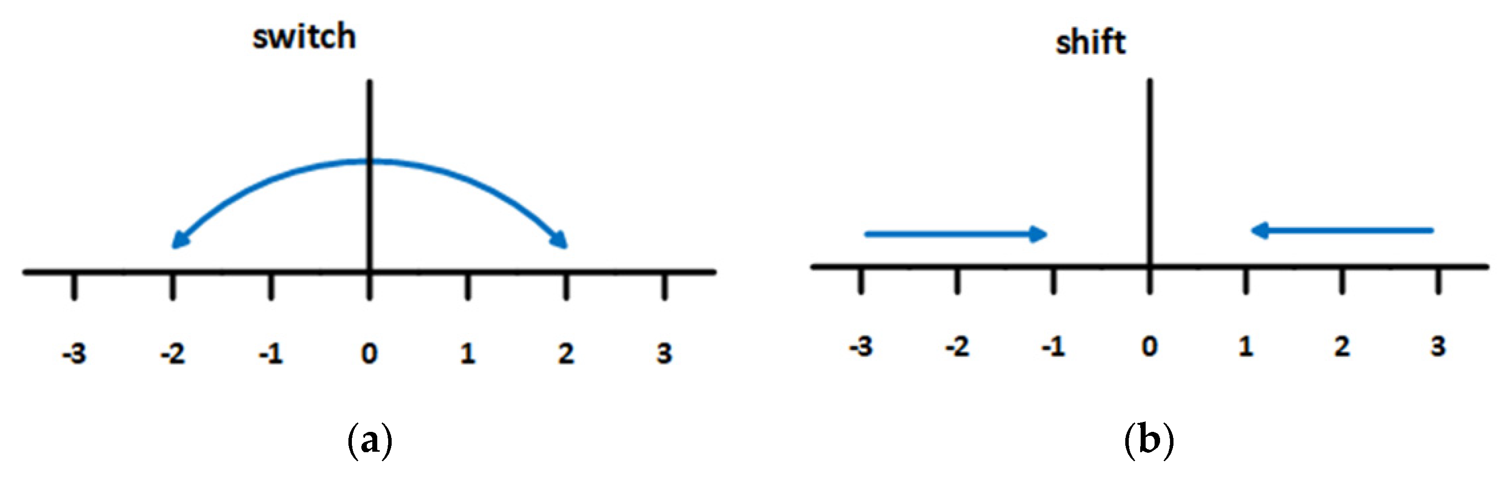
In our approach, negations are processed in a new way, using the interactivity of switch and shift negation [
26]. Switch negation only turns polarity to its opposite (e.g., from +2 to −2), as illustrated in
Figure 6a. Shift negation is more precise than switch negation, only shifting the polarity of a connected word towards the direction to opposite polarity, as illustrated in
Figure 6b.
We designed the interactive so-called ‘combined negation processing’, where shift negation is applied to extreme values of polarity of connected words (+/−3) and switch negation is used for processing most obvious polarities (with absolute value
1 or
2). The combined approach significantly increases the effectivity of opinion classification, as illustrated in
Table 12.
After involving intensifiers and negations, the polarity of the whole post is not calculated using the simple approach (9) but, instead, using the new approach (11):
where
Pp is the post’s polarity,
Pw is the word’s polarity,
∏Pi is the multiplication of polarity of words by intensifiers in a post, and
∏Pn is the multiplication of polarity of words by negations in a post.
7.1. Topic Identification in Opinion Classification
Another method that we used to increase the effectiveness of the opinion classification was involving topic identification. Topic identification can be helpful in increasing the influence of a text of post concentrated on the topic of an online discussion. Polarity of these posts was increased using greater weights. We tested two methods for topic identification: Latent Dirichlet Allocation (LDA) and Term Frequency (TF). LDA is a standard probabilistic method, based on the Dirichlet distribution of probability of topic for each post. In the output of the LDA, there is a list of words accompanied with their relevancy to all texts in the data set (so called topics). An experiment was carried out, with all texts in the data set processed using LDA. The output was a list of 50 words relevant to topics present in the texts. As there were too many “topics”, the list was reduced to 15 words with the highest relevancy to the topics of the processed texts.
The second method was topic identification based on the term frequencies of words in posts. We assumed that the words in posts relevant to the topic of online discussion should have higher occurrence in these texts. A disadvantage of this method is the highest occurrence of stop words in texts. For this reason, stop words must be excluded in pre-processing. We did not create this list, instead using a known list of stop words.
First, the opinion polarity of posts was estimated. In the second step, words relevant to the identified topic of discussion were searched for in the post. If such words were found in the post, then the opinion polarity of the post was increased (by multiplication with value 1.5). The value of 1.5 was set experimentally, after experiments with three values: 1.5, 2, and 3. The double and triple changes of polarity led to slight decreases in the quality of the results obtained. Results of experiments with topic identification in the opinion analysis are illustrated in
Table 13.
The results of the experiments, as presented in
Table 13, show that the implementation of topic identification increased the Precision and Recall of the opinion classification of posts in online discussions. Topic identification using LDA achieved better results than using the term frequency method. People often express negative opinions while talking about the main topic. This negative opinion is usually compensated for by more positive posts related to less important aspects of the discussed problem. In this case, topic identification can significantly increase the precision of opinion classification.
7.2. A Hybrid Approach to Opinion Classification
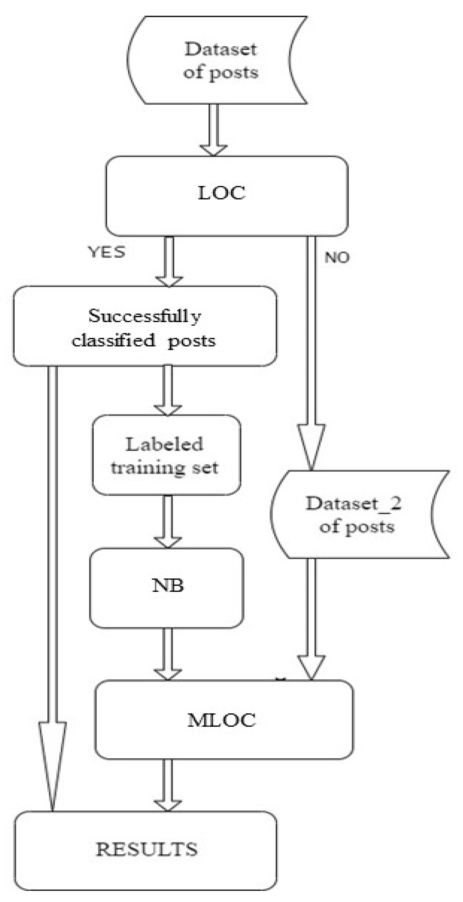
The proposed hybrid approach to opinion classification combines the advantages of two different techniques for an opinion classification model creation. The first technique is the lexicon-based approach, which is simple and intuitive; however, it can fail when the lexicon is not sufficiently expressive. The second technique—The machine learning approach—Does not depend on the quality of the lexicon, but requires a labelled training set as an input for training an opinion classification model. Therefore, we designed the hybrid approach to increase the effectiveness of the opinion analysis of posts when the lexicon approach fails (see
Figure 7). The posts which were successfully classified as having positive or negative opinion using the lexicon (and, in this way, were labelled) were put into the training data set, in order to train a probability model based on the Naive Bayes machine learning method. This model was then able to classify posts that did not contain words from the lexicon and could not be classified using the lexicon approach.
At first, Lexicon-based Opinion Classification (the “LOC” block) is applied to classify all posts in the data set. Once all posts are classified either successfully (YES) or unsuccessfully (NO), the dataset is split into two groups: labelled and unlabelled posts (Dataset_2). Labelled posts represent the training set, which is used for Naïve Bayes model training (the “NB” block). The trained Naïve Bayes model is then applied to classify posts in Dataset_2 which were not classified by Lexicon-based Opinion Classification; this is the “MLOC” (Machine Learning Opinion Classification) block. All classified posts, as classified by LOC and MLOC, are then saved (the “RESULTS” block).
The hybrid approach for opinion classification was tested and compared with the original lexicon approach. The results of testing are presented in
Table 14, in the form of F1 rate—particularly, F1 Positive (F1 rate on positive posts), F1 Negative (F1 rate on negative posts), and Macro F1 rates—on the General data set. The results in
Table 14 show a strong increase of efficiency, as measured by F1 rate, when the hybrid approach for opinion classification was used. The reason for this increase of efficiency can be explained by decreasing of the number of unclassified posts. The unclassified posts decreased the precision of classification, as positive and negative posts were classified to neutral ones due to absence of positive or negative words in the lexicon. Using the hybrid approach, the number of unclassified posts was reduced from 18% to 0.03%. In future research, we would like to use deep learning [
35] for the machine learning-based opinion analysis method in the hybrid approach.
The complexity of the lexicon approach for opinion classification is , thus being linear in the size of posts in the training set M and the size of lexicon D. The complexity of the machine learning approach for opinion classification using the Naive Bayes algorithm is , thus linearly depending on the total number of posts in the training set M and the number of attributes (words) in the training set N. It follows that the complexity of the hybrid approach is .
8. Discussion
The main purpose of this paper is to find the best method for labelling a lexicon for a lexicon-based approach to opinion classification. Therefore, it is natural that our baseline was the lexicon-based approach, not a machine learning approach. This is the reason for comparison of the effectiveness of the hybrid approach with the lexicon approach as a baseline. This basic lexicon approach was extended by a machine learning approach, in order to achieve better results in the case when the lexicon could not overlay texts using another dictionary.
It was not our goal to test all machine learning methods but, instead, to discover whether a supplementary model trained by machine learning can decrease the number of failures in the opinion classification of problematic texts. The use of Naïve Bayes was a natural choice, as this method also gives weights to words (i.e., labels) in the form of a conditional probability of the word belonging to a given class in the data. Deep learning also trains the weights of attributes (words, in this case), but clear information about these weights is lost due to the large number of inner layers used. In the field of text processing, we also often use Random Forest or kernel SVM methods. However, these machine learning methods do not provide intuitive and explainable solutions with clear information about the measure of sensitivity of words in a model either.
The findings of the presented work are useful for our research in the field of antisocial behavior recognition in online communities and in the field of human–robot interaction. Our approach can provide the results of opinion and mood analysis of texts for use in these fields. The presented work is focused on opinion classification using a lexicon approach and, so, we needed to generate a high-quality lexicon using effective labeling.
In this paper, an automated method for lexicon labelling was proposed. It used nature-inspired optimization algorithms—Particle Swarm Optimization (PSO) and Bare-bones Particle Swarm Optimization (BBPSO)—to find optimal polarity values for words in the lexicon. The results of numerous tests on two data sets (Movie and General) were provided and presented in the paper. These tests showed that BBPSO labelling is better than PSO labelling, and that both are better than human labelling. Two lexicons (Big and Small) were created, in order to achieve good performance, which were labelled by both PSO and BBPSO. The experiments showed another finding: the human annotator avoided labelling words with a number close to zero, whereas PSO or BBPSO assigned zero values to some words.
We tested the labelling of lexicons using our new lexicon approach. The novelty of this approach comprised a new approach for intensifier processing and an interactive approach for negation processing. This new approach also involved topic identification and a hybrid approach for opinion classification, using not only lexicon-based, but also machine learning-based opinion classification methods. The hybrid approach was applied to classify the posts which were not classified by the lexicon approach.
For the future, we would like to extend our automatic lexicon labelling to learn polarity values representing the concept-domain pair. In some cases, the polarity of the word can be different in different domains. In that case, the polarity value represents the polarity of the word in the given domain. Furthermore, we would like to focus on the statistical analysis of words labelled by PSO and BBPSO, respectively. On one hand, the optimized labels will be compared with human labelling. On the other hand, removed words (i.e., the words labelled with zero) will be analyzed deeper, in order to answer the following questions: Which words were removed from the lexicons? How often are they removed?
The final hybrid model for sentiment analysis can be used in our research in the field of emotion analysis in human–robot interactions, where understanding of human mood by a robot can increase the acceptance of a robot as an assistant.
We are also using our work in sentiment analysis in the field of recognition of antisocial behavior in online communities. We would like to model the sentiment and mood of society in connection with the phenomenon of CoViD-19 [
36].


