1. Introduction
As the framework of a city, road networks have attracted the concern of scholars in all aspects of urban research and are regarded as one of the five major elements in city construction by Lynch (1960) [
1]. The pattern of urban road network is complex and diverse, which reflects the characteristics of road distribution and the political, economic, and cultural characteristics of a city in a particular historical period [
2,
3,
4]. It is crucial to accurately identify road patterns for road navigation, urban planning, and functional zoning. Therefore, accurately identifying the road patterns in complex road networks have become the focus for GIS research [
5].
In urban road networks, the overpass is one of the most important road patterns. An overpass as a three-dimensional cross bridge in a road network refers to a modern building that is built on the intersection of two or more intersecting roads with different levels and different directions. Its main function is to make the vehicles in all directions free from traffic lights at the crossroads so as to pass quickly. Scheiders proposed an identification method for an overpass based on road attributes [
6], but actual road data may have only partial or incomplete attribute information, such as OpenStreetMap (OSM) road data [
7]. In contrast to attribute information, geometric features are more essential to road networks, so how to identify an overpass using geometric features becomes a problem.
In recent years, an overpass is mainly identified by traditional vector-based methods coming from computational geometry and graph theory. Mackaness and Macchechnie proposed a method to identify and simplify unstructured overpasses [
8]. In their method, an overpass was firstly positioned by searching for the denser node areas in road networks, and then the hierarchical relationship between the sections of local road network was constructed. Finally, the structure of the overpass was simplified by a graph simplification method. However, since the internal structure of an overpass is too complex to be accurately identified by their method, which can generate many wrong simplified results, it is necessary to manually judge whether the results are correct. In 2011, Xu proposed an overpass identification method based on structural patterns [
9]. In his method, the structure of the road intersection was described using a directional attribute relationship graph, the template library of a typical structure was established and correspond intersections were identified using a relationship graph described by the template. Compared with the method proposed by Mackaness and Macchechnie, the accuracy of the identification results was improved. However, this method relies too much on artificially constructed structural templates and is hard to apply to atypical overpasses. In 2013, Qian proposed an improved structural pattern recognition method [
10]. In his method, road topological features were used to describe an overpass, a typical quantitative expression template library was established, and the overpass was identified by comparing the structure with quantitative expressions. In 2016, Ma proposed a method to enrich the structure description in his previous papers [
11]. An overpass feature space was established by using six parameters, including length, area, compactness, parallelism, symmetry, and semantic attributes. Then a support vector machine (SVM) was trained and used to identify the main roads and auxiliary roads in each overpass. However, his method cannot identify the overall structure of an overpass directly.
The above methods belong to the identification approach based on artificially designed features. The overpass structure is mapped to a feature description space through spatial calculation, and then the overpasses are identified and classified. Such methods rely too much on the design of the feature items (such as length, angle of intersection, curvature, graph template, etc.). These artificially designed shallow features only work well for standard overpass structures in an ideal state. However, in actual data, an overpass is often under an unsatisfactory state, and there are many disturbing factors. In order to identify overpasses in actual data more accurately, Qian and He proposed to solve the overpass classification problem by a machine learning method in 2018 [
12]. In their method, a convolutional neural network (CNN) was trained with images containing overpasses to classify them into different types. Artificially designed feature items were not needed, instead, road data was converted into raster data as the training data for the CNN model. Their method combines vector data and raster images, and uses the neural network learn the fuzzy characteristics of overpasses, and classifies the complex overpass structures in OSM. As far as we know, this method is the first attempt to classify overpasses using a CNN model. In the classification process, feature items are not needed to be given manually, and the uncertainty of the result is reduced by the self-learning mechanism. However, his method can only be used to classified the types of overpasses and cannot be used to identify the location of overpasses in a large range of road networks.
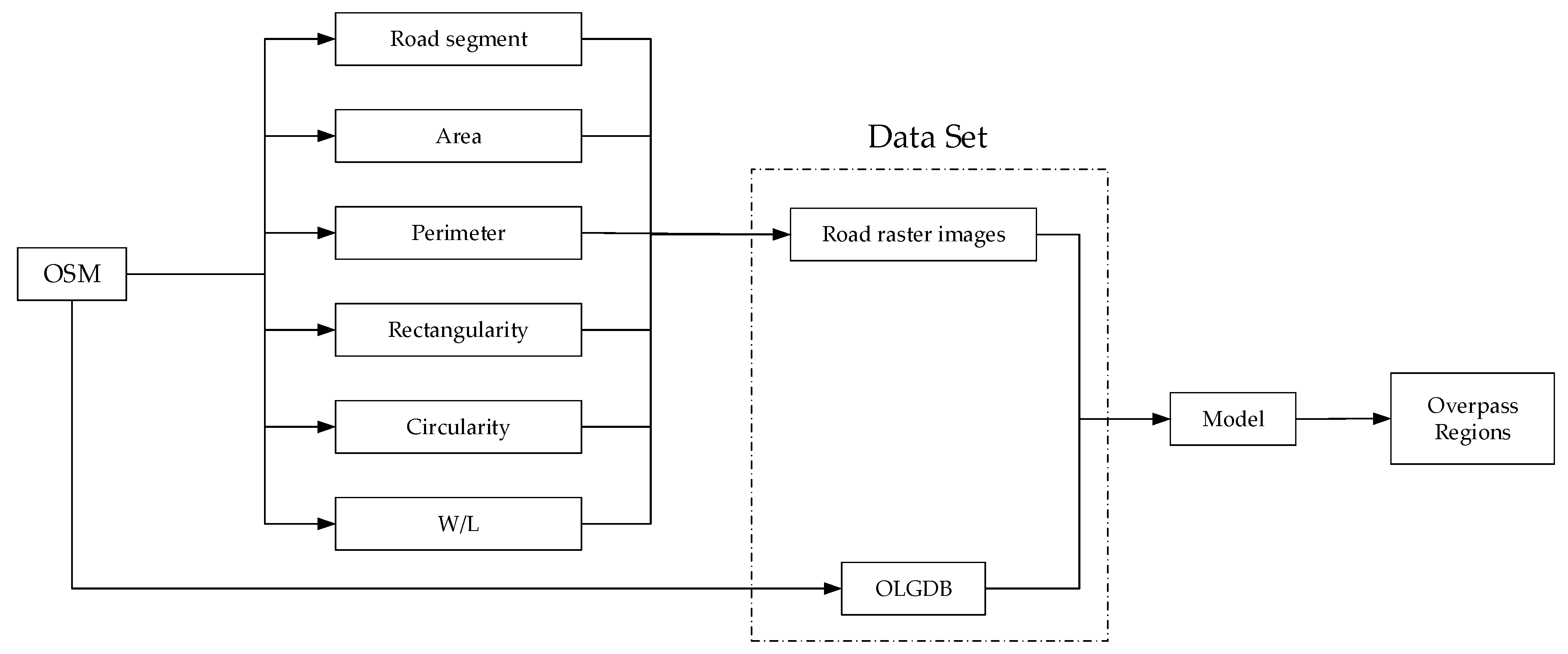
In order to handle the location problem mentioned above, this paper aims to identify overpasses in road networks using a target detection model of deep learning (Faster-Region Convolutional neural network, Faster-RCNN). As there is no labelled data for such problem at present, an overpass labelling geodatabase (OLGDB) for the OSM road network data of six typical cities in China was established. The data flow chart is shown in
Figure 1.
In the training data generating phase, we integrated five geometric metrics of roads into image bands and further compared the contribution of these metrics. Finally, three geometric metrics having better effects were selected to be synthetized into the RGB band values in order to use pre-trained CNN models. Three different CNNs (ZF-net, VGG-16, Inception-ResNet V2) were integrated into the Faster-RCNN model and evaluated to find the optimal one by accuracy performance. The results of different model parameters (such as learning rate, batchsize) were measured by fine-turning experiments. The experimental results showed that Faster-RCNN can be applied to the identification of overpasses and good results were achieved. This work can be used to evaluate and supervise the development of urban road networks which is significant in urban science.
2. Research Method
In the field of computer vision, image classification and detection are the focus for research [
13,
14]. An image classification model is used to divide each image into a single category, usually corresponding to the most prominent object in the image [
15,
16,
17]; but in the real world, in general, images do not only contain one object, so it is not accurate to simply assign images to a single label. For such a case, a target detection model is needed and used to identify multiple objects in an image and to determine the position of objects in images using rectangular bounding boxes [
18,
19,
20]. So, in this paper, Faster-RCNN, which meets the above requirement, is studied to identify overpasses in road networks.
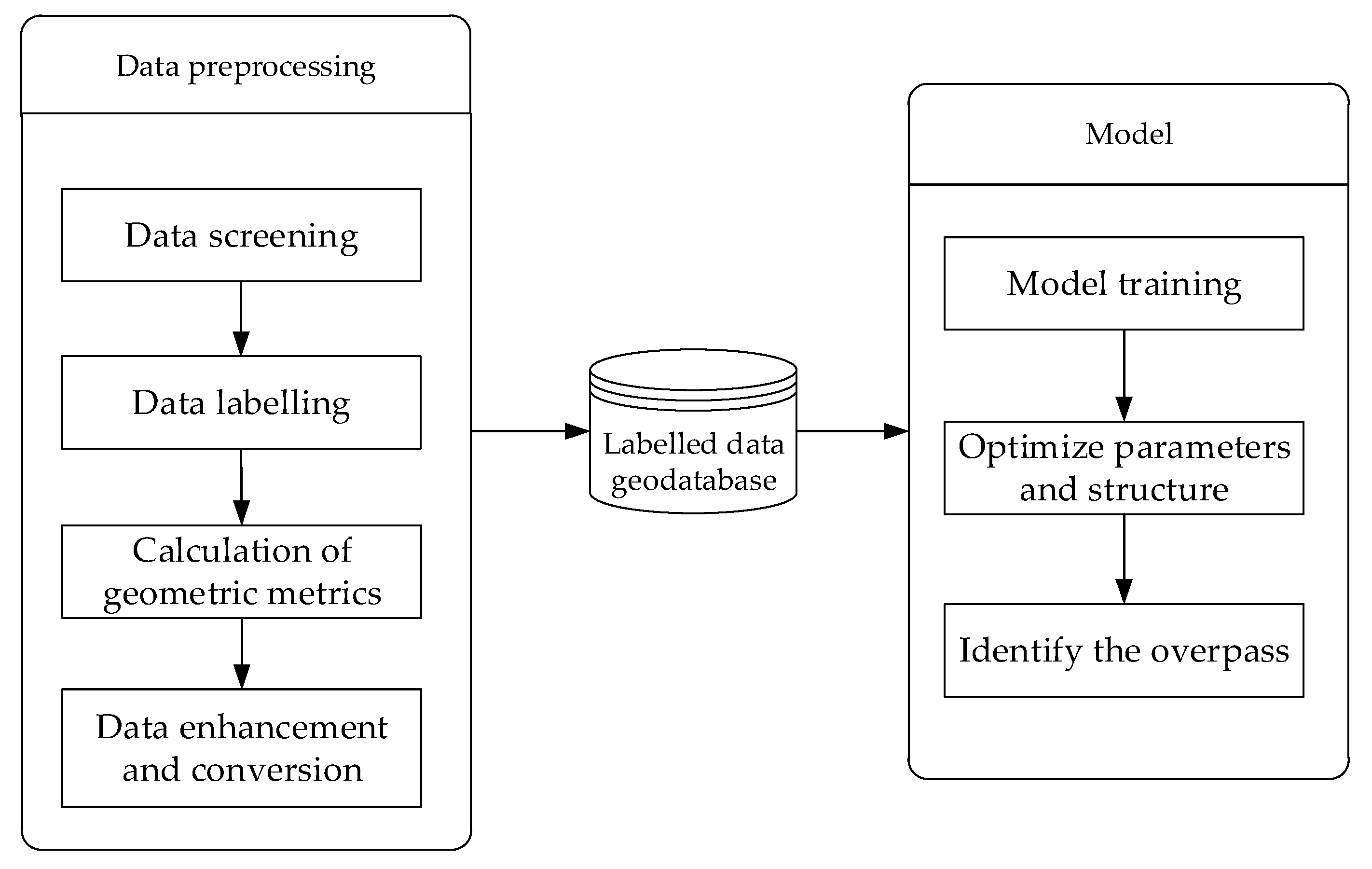
The research route is as follows, firstly, OSM road network data is preprocessed (mainly including data screening, data labelling, calculation of geometric metrics, data enhancement and conversion) in order to generate the training data needed by the model. Then, training data is used to train Faster-RCNN and the model parameters and structure are optimized through contrast experiments. Finally, the optimal model is used to detect road networks and overpasses are marked using a rectangular bounding box. The technical flow chart is shown in
Figure 2.
2.1. Data Preprocessing
The data source for this paper is OSM road data. OSM is an online map collaboration designed to create a free world map that everyone can edit [
21,
22]. So OSM data is a typical kind of volunteered geographic information (VGI) data, which can be voluntarily contributed by anyone who wants to: children or adults, amateurs or experts, they may have different motivations and may even be contributing without their knowledge [
23,
24]. Data contributors use satellite images, GPS devices, and traditional regional maps to ensure accuracy and timeliness.
There are many advantages of OSM, such as short update periods, convenient data acquisition access, and good data quality [
25]. These characteristics make OSM data an ideal source for many scientific research experiments. The utility of OSM has been studied as a potential source of road data and the results have been promising [
26,
27]. Thus, OSM road data is selected as the data source for this paper.
2.1.1. Data Screening
In OSM data, road data has a type attribute (Fclass) which represents the category of roads and includes attribute values such as motorway and step [
28]. Before an overpass is labelled, road data is filtered according to the Fclass attribute, which aims to eliminate some irrelevant data such as pedestrian bridges and tunnels. Compared with the initial data, filtered road data is more significant, which is beneficial to the study of Faster-RCNN on the focus of overpass structures. Parts of valid Fclass attribute values of OSM road data are shown in
Table 1:
2.1.2. Data Labelling
In this paper, an OLGDB is established to store all the labelled overpasses which were produced by ArcGIS software on a OSM road network and confirmed by Google Maps. Overpass structures are labelled with vector polygons rather than rectangular bounding boxes (a traditional target detection task is to select an object in images as a positive sample using a rectangular bounding box). This facilitated subsequent data enhancement operations:
The illustration of the above two reasons is shown in
Figure 3.
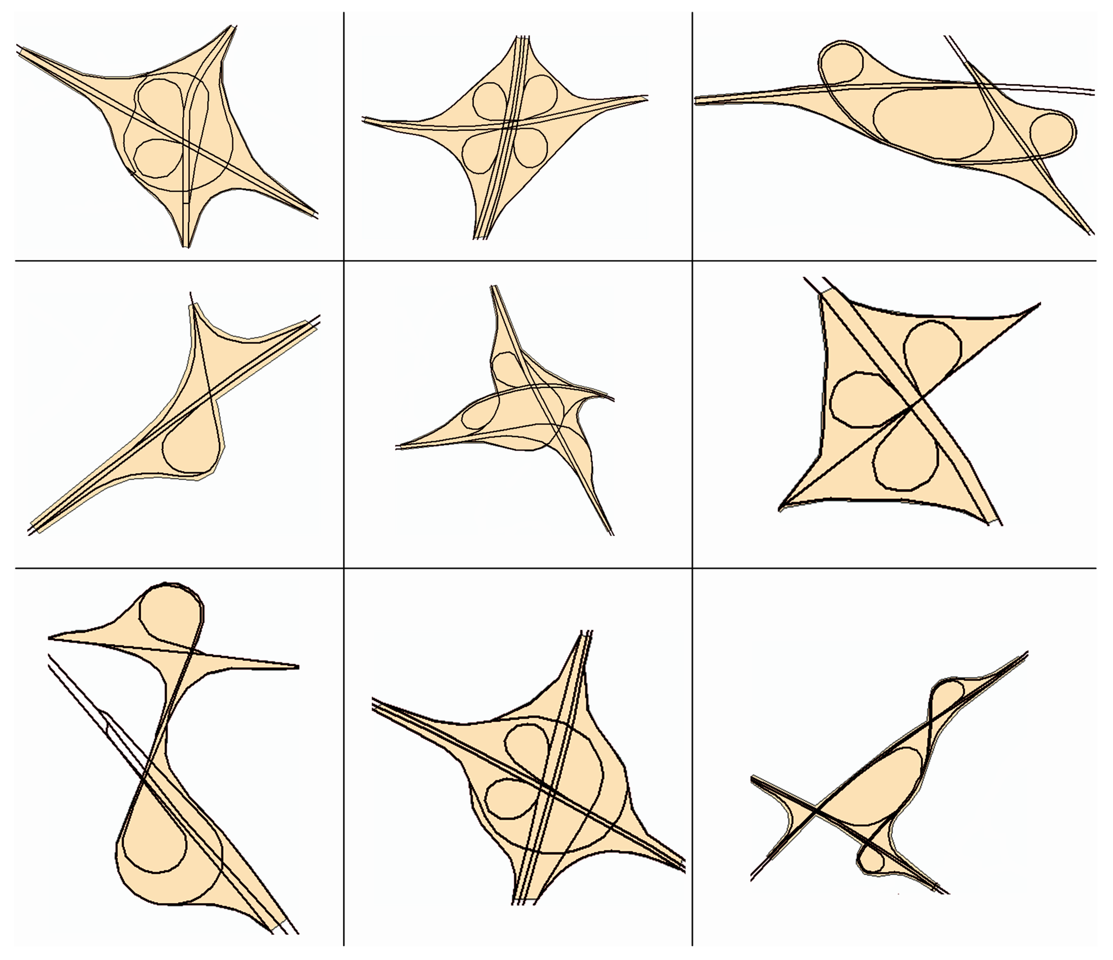
There are 640 labelled overpasses in the OLGDB, part of them are shown in
Figure 4.
2.1.3. Calculation of Geometric Metrics
In the generation of training data, geometric information is only partially kept with the conversion from vector to raster. So geometric metrics which measure morphology diversities in field form need to be included to enhance the presentation ability. Five different geometric metrics, including perimeter, area, squareness, circularity, and W/L (the width to length ratio of the circumscribed rectangle), are calculated. Three of them with better effects are selected as the RGB band values of training data through experiment comparison, corresponding to the 3D input variant of pre-trained CNN structures in Faster-RCNN.
The polyline-based network skeleton model is converted to a polygon-based street block model by ArcGIS in order to get the five geometric metrics. The perimeter and area of the block surrounded by road sections can be obtained directly.
Rectangularity is the ratio of block area to the area of the MER, reflecting the filling degree of a block to its MER. The formula is as shown in Equation (1):
where
is the rectangularity of a block,
is the block area and
is the MER area of a block.
is between 0 and 1. The more curved the block, the smaller the rectangularity.
Circularity is an important geometric metric in image processing and it can be used to describe the closeness of a polygon to a circle. The circularity of a circle is 1. The smaller the circularity, the more irregular the image and the larger the gap with circle. The calculation formula of circularity is as shown in Equation (2):
where
is the block area and
is the block perimeter.
W/L is the width to length ratio of the MER. W/L is used to distinguish an elongated block from a round or square block. The calculation is shown in Equation (3):
where
represents the width of the MER and
represents the length of the MER.
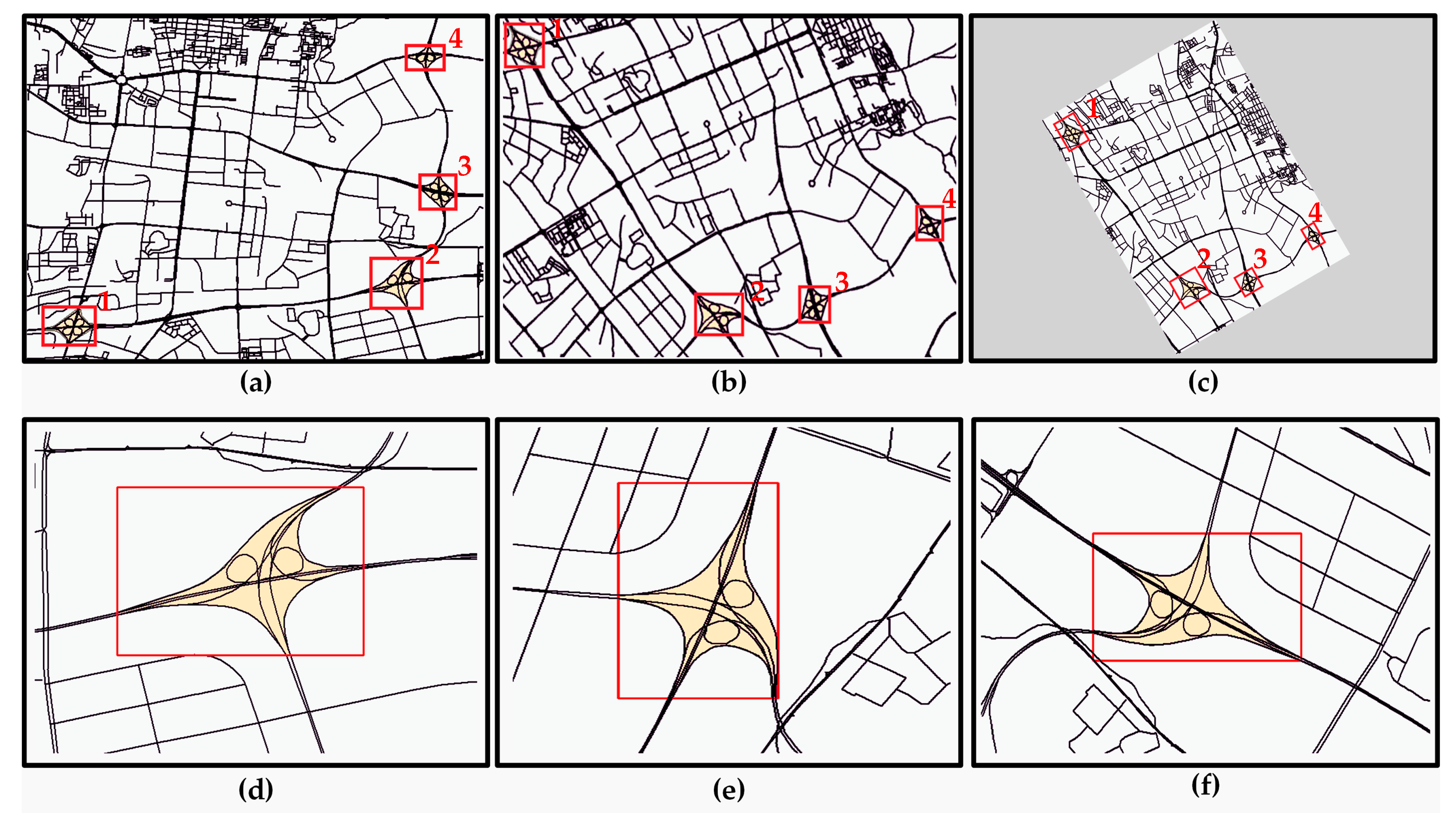
2.1.4. Data Enhancement
Deep learning models require a large amount of training data to ensure accuracy, but the overpasses in road networks are relatively sparse, so two kinds of data enhancement are employed to amplify the training data. The first type of data enhancement is to enhance the overpass and its description polygon by vector rotation conversion. After the overpass vector data is rotated, the relative coordinates of positive samples will change. The coordinate variation formula of rotation conversion is shown in Equations (4) and (5):
where
and
are converted coordinates and
α is the angle at which vector data rotates clockwise.
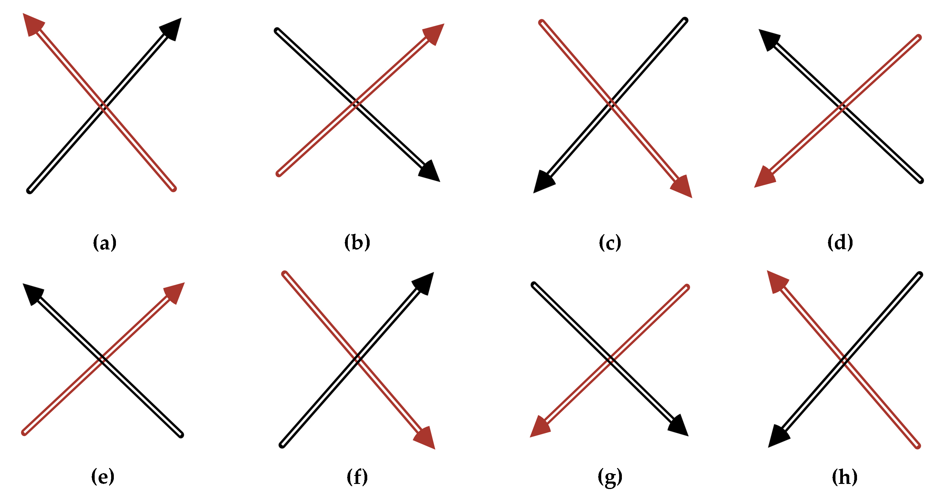
The second type of data enhancement is to enhance the converted raster data. There are eight patterns for an image, as shown in
Figure 5.
Therefore, we rotate and flip each training image to generate eight images with different axis change rules. When an image undergoes the above-described rotation and transposition, the size of the image remains unchanged, the information in the image is not lost. This not only ensures the accuracy of the training data, but also increases the sample number of overpasses. After the image data is enhanced, the relative coordinates of overpass structure in each training image are obtained by coordinate conversion formula. Coordinate conversion formulas are as shown in Equations (6)–(13) (taking the form of
Figure 3b,e as examples):
The boundary coordinates of the positive samples in the training image of
Figure 3b are obtained by Equations (6)–(9),
,
,
,
represent the upper-left and lower-right coordinates of the positive sample region in
Figure 3b,
,
,
,
represent the upper-left and lower-right coordinates of the positive sample region in the initial configuration; the boundary coordinates of the overpasses in the training image of
Figure 3e are obtained by Equations (10)–(13). Width represents the width of training image. After the above data enhancement, the problem that the training data is rare can be solved as 12,000 training images can be provided to the learning model.
2.1.5. Data Conversion
After three geometric metrics with better effects are selected (as described in
Section 2.1.3), the values of the geometric metrics are adjusted to 0–255 space, and then, the data conversion function of the Geospatial Data Abstraction Library (GDAL) is used to convert vector road data to raster and to keep adjusted geometric metrics in RGB bands of raster images. GDAL is an open source raster spatial data conversion library under the X/MIT license, which uses an abstract data model to access various geodata file formats and also has a series of command-line tools for data conversion and processing. The converted raster images are shown in the
Figure 6.
2.2. Target Detection Model
This paper aims to identify overpasses in road networks using a target detection model of deep learning (Faster-RCNN). In Faster-RCNN, a convolutional neural network (CNN) is used to extract road features and generate feature maps; the backend contains RPN and ROI pooling; it can generate, adjust, and classify regions.
2.2.1. Convolutional Neural Networks
A convolutional neural network (CNN) is a feedforward neural network and its artificial neurons can respond to a part of surrounding areas. It has excellent performance for large image processing [
29]. A CNN consists of one or more convolutional layers, fully connected layers, and pooling layers. This structure enables the convolutional neural network to take advantage of the two-dimensional structure of input data. CNNs give better results in image and speech recognition tasks than other deep learning structures, and can also be trained using backpropagation algorithms [
30]. Compared with other depth and feedforward neural networks, CNNs require fewer parameters, making it an attractive deep learning substructure.
CNN provides an end-to-end learning model for image feature extraction and learning. The parameters in the model can be trained by traditional gradient descent methods. Trained CNN can learn features in image and can extract and classify those features. As an important research branch in the field of neural networks, CNN is characterized by the features of each layer being calculated by the local region of the upper layer through the sharing of the convolution kernel of weight. This characteristic makes CNN more suitable for learning and expressing image features than any other neural network architectures.
In a CNN, the convolution calculation is performed by a sliding mechanism and convolution kernel. The elements of a convolution kernel matrix and the elements of a covered area are multiplied and accumulated. Each convolution kernel is a feature extractor, and the convolution operations at all locations in training images share the weight of convolution kernel. In general, in a target detection model, a single convolution kernel is not sufficient, and multiple convolution kernels are needed to extract different levels of features in training images. In a CNN, the features of training images are stored in the form of feature maps. Assuming that the
j-th feature map of the
l-th layer is
, then the convolution calculation of
is as shown in Equation (14).
where
is the weight parameter of convolutional layer,
is the bias variable parameter, and
is the activation function, which is used to apply nonlinear transformation on input values.
In order to reduce the size of parameters, there can be a pooling layer after convolutional layer. The role of the pooling layer is to reduce the size of the feature map. Assumed that the feature map after pooling is
, the calculation formula of pooling operation is as shown in Equation (15).
where
is the weight parameter of the pooling layer,
is the bias variable parameter and
is the pooling operation types. For example, when the size of the pooling layer is set to be 2 × 2 and the type of pooling operation is “MAX”, it means that the pixel value in the range of 2 × 2 is replaced by its maximum value.
is the activation function.
There are a variety of CNNs, such as the classic LeNet-5 model, which are mainly used in some fundamental computer vision applications, such as handwritten character recognition and image classification. The Convolutional Deep Belief Network that is generated from a CNN and Deep Belief Network has been successfully applied to face feature extraction as an unsupervised generation model [
31,
32,
33]. A Full-convolution network (FCN) realizes end-to-end image semantic segmentation and greatly surpasses traditional semantic segmentation algorithm in accuracy [
34]. Alex Net has achieved breakthroughs in the field of massive image classification [
35]. RCNN based on region feature extractions has achieved success in the field of target detection [
36]. The target detection model used in this paper is the Faster-RCNN model under the RCNN series model.
2.2.2. Faster-RCNN Model
The Faster-RCNN model is a deep learning target detection model [
37]. It uses CNN as a substructure and greatly improves the effect of target detection. It is a two-stage detection algorithm. This algorithm divides the detection problem into two phases:
The structure of Faster-RCNN model is shown in
Figure 7.
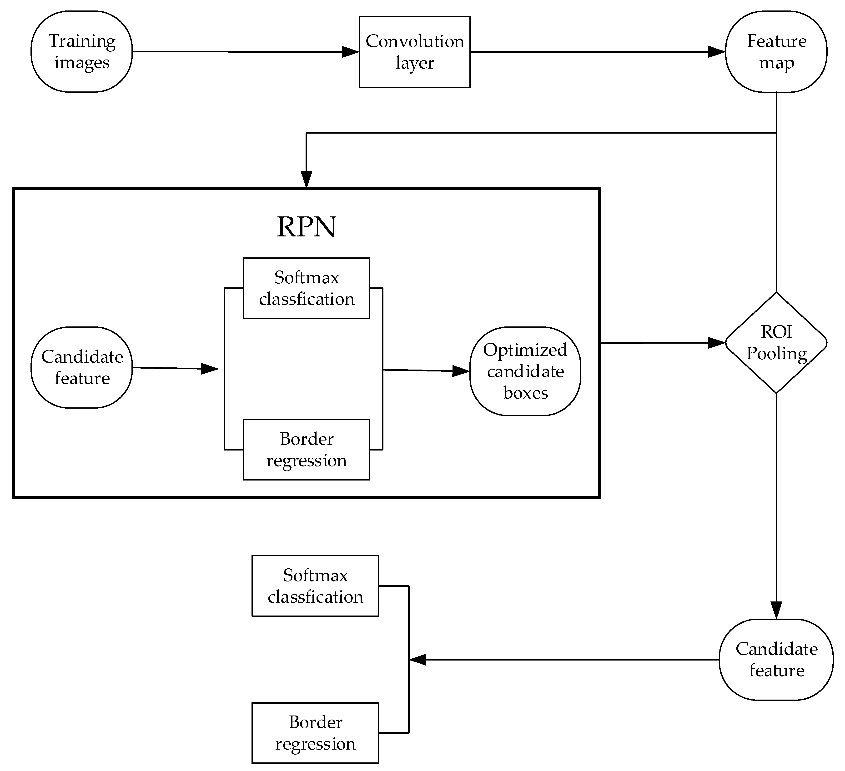
The Faster-RCNN model is an improvement of the Fast-RCNN model. In the Fast-RCNN model, the generation of candidate regions is realized by a selective search algorithm, which is a very time-consuming process. The Faster-RCNN model is improved on this point and the Region Proposal network is introduced to generate candidate regions, namely Faster-RCNN = Fast-RCNN + RPN [
38]. In the Faster-RCNN model, the feature map of an image is firstly generated by CNN, and then the generated feature map is input into the RPN network. The RPN network obtains candidate regions and enters them into the ROI pooling layer. The ROI pooling layer receives both the optimized candidate boxes of RPN output and feature map of convolution layer output, then the regions in the feature maps corresponding to the optimized candidate boxes are pooled.
The corresponding features of candidate regions are extracted in feature maps. Finally, two fully connected layers are entered, one is the classification layer (Softmax classification), which is a multi-objective classification layer, giving each candidate region a category label, and the other is the coordinate regression layer, which can be used to adjust the coordinates of the candidate areas.
In the RPN network, features are extracted from feature maps using a sliding window, and each sliding window generates k candidate regions with different sizes and different aspect ratios (generally using 3 different sizes and 3 different aspect ratios, i.e., k = 9). Next, the corresponding feature of each candidate region is input to two fully connected layers. One is a classification layer (Softmax classification). This classification layer performs binary predictions to determine whether each candidate region is an object. The other is the coordinate regression layer, which is used to adjust the coordinates of candidate regions. The RPN network shares the same group of convolutional layers with Fast-RCNN. This strategy can simultaneously train and adjust the RPN network and Fast-RCNN. Therefore, the Faster-RCNN model becomes a completed end-to-end model, and the training speed and detection accuracy of the model are greatly improved.
For training RPN, if a candidate region is one of the following two cases, the label of the candidate region is positive.
Note that a single ground-truth box may assign positive labels to multiple candidate regions. Usually the second condition is sufficient to determine the positive samples; but the first condition must be considered for the reason that, in some rare cases, the second condition may find no positive sample. The label of a candidate region is negative if its IOU is lower than 0.3 for all ground-truth boxes. Candidate regions that are neither positive nor negative do not contribute to the training objective.
In the Faster-RCNN model, the loss function is defined as shown in Equation (16).
The loss function has two parts. The classification loss
is log loss over two classes (object vs. not object),
i is the index of a candidate region,
is the predicted probability of region
i being an object. The ground-truth label
is 1 if the candidate region is positive, and is 0 if the candidate region is negative. The other one is the regression loss,
is a vector representing the four parameterized coordinates of the predicted bounding box, and
is that of the ground-truth box associated with a positive region. For boundary box regression, we use Equations (17)–(20) to calculate the coordinates.
where
x,
y,
w, and
h denote the box’s center coordinates and its width and height. Variables
x,
, and
are for the predicted box, region box, and ground truth box, respectively (likewise for
y,
w,
h).
3. Experiment and Result Analysis
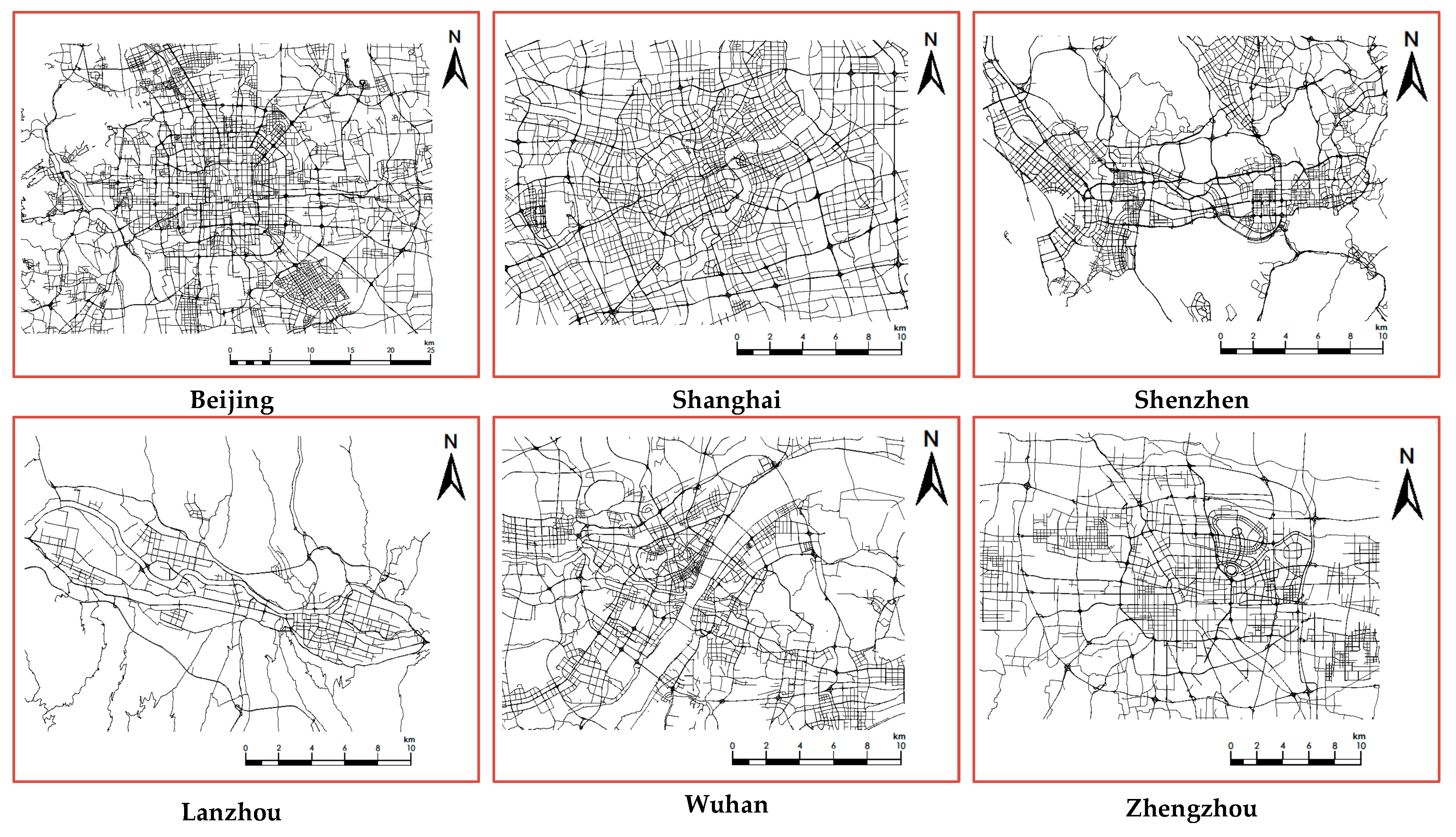
In this paper, Beijing, Shanghai, Shenzhen, Wuhan, Zhengzhou, and Lanzhou in China were selected as the experimental research areas. Beijing, Shanghai and Shenzhen were selected as representatives of first-tier cities. Beijing is the capital of China and its urban roads are all in a chessboard pattern. By the end of 2018, the city’s highway mileage was 22,255.8 km. Shanghai as a municipality directly under the Central Government of China is located in the Yangtze River Delta with a highway mileage of over 16,000 km. Shenzhen is one of the four first-tier cities in China. It is located in the southern Guangdong Province and is a national transportation hub city. Wuhan, Zhengzhou, and Lanzhou were selected as representatives of second-tier cities. Wuhan is located in the central part of China and the Jianghan Plain in eastern Hubei Province. The highway mileage exceeds 15,000 km. Zhengzhou is an important central city in central China, with a total main highway length of approximately 12,700 km. Lanzhou is one of the important central cities in western China and a transportation hub in the northwest. These cities, as representatives of China’s first- and second-tier cities, are located in different parts of China, which makes research data more representative and diverse. The road data for the selected cities are shown in
Figure 8.
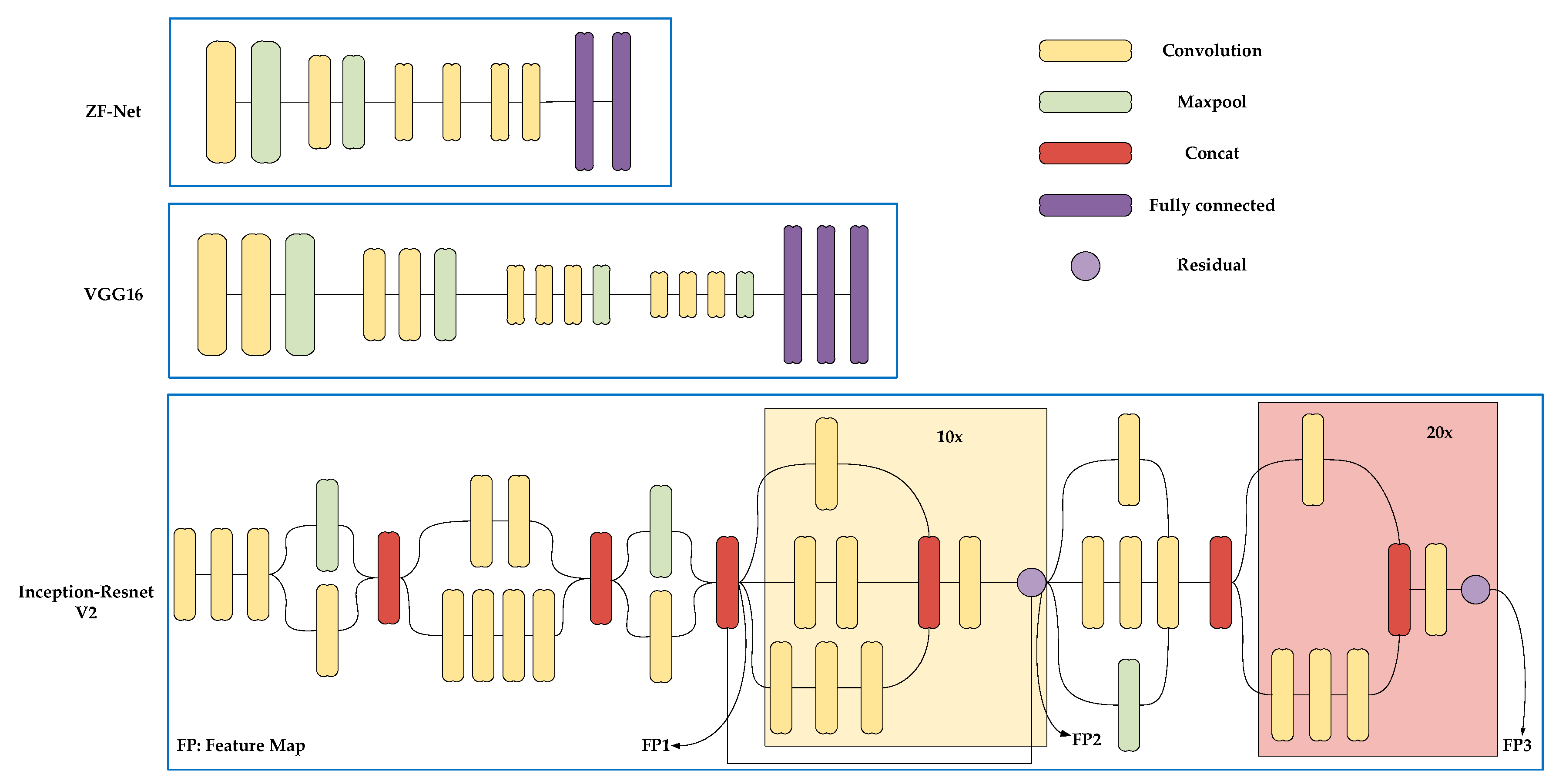
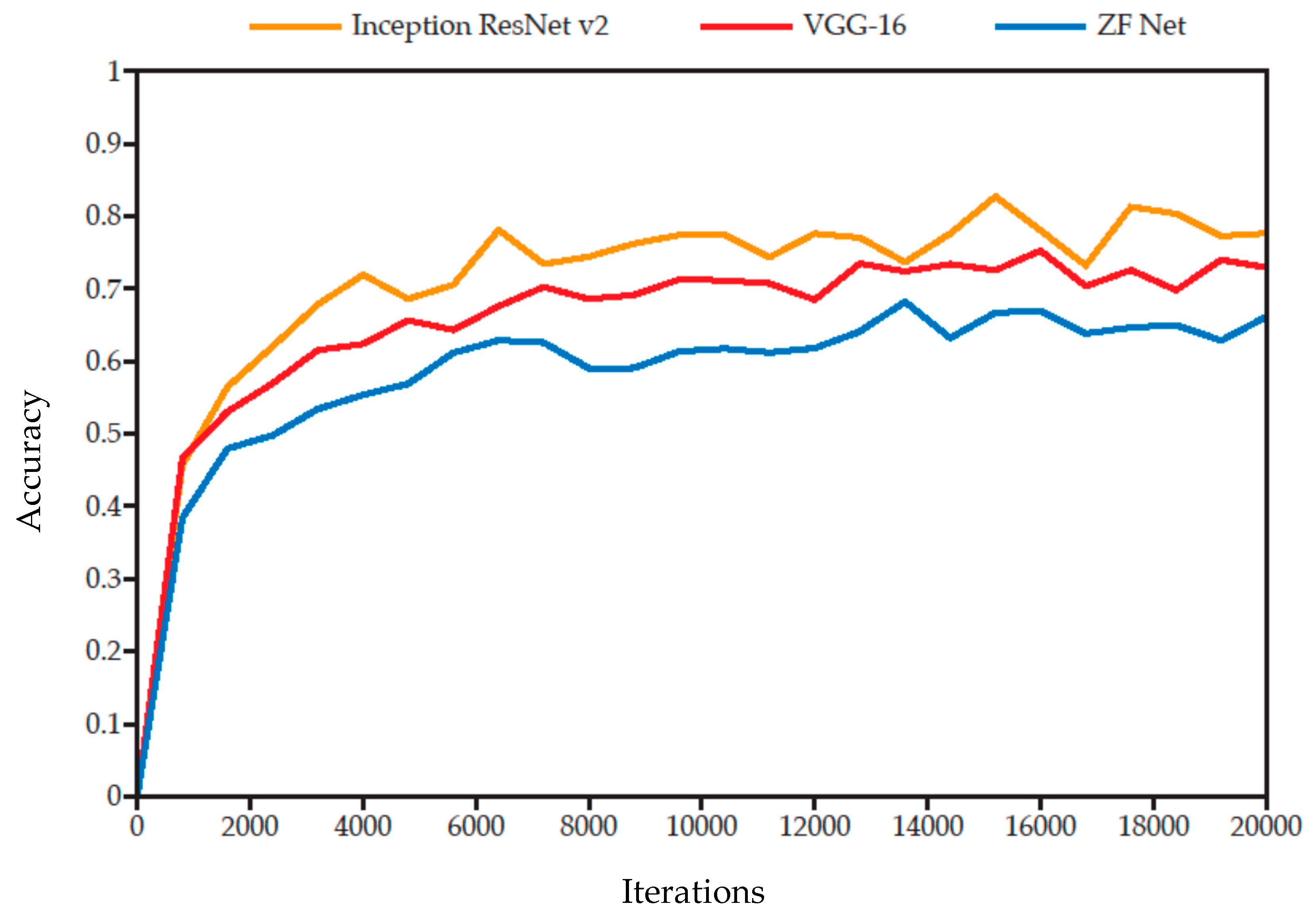
In this paper, a series of comparative experiments are designed and conducted to study the influence of different geometric metrics, model structures, and model parameters on the overpass identification task. Experiment 1 tests the distinct effects of CNN substructure. We integrated three different CNNs (ZF-net, VGG-16, Inception-ResNet V2) into Faster-RCNN. These convolution structures are normally used to accomplish feature extractions. In addition, they have better performance in feature extraction for complex structures because of their sophisticated layer design. The three CNNs are shown in
Figure 9.
ZF-net consists of five convolution layers and two fully connected layers [
39]; VGG-16 has 16 total convolutions and fully connected layers [
40]; Inception-ResNet V2 introduces two special modules: Inception and residual [
41]. In inception modules, multiple convolution branches are linked to a single feature map, while residual modules (those that repeat 10 or 20 times in Inception ResNet V2 in
Figure 6) add input feature maps to the convoluted output.
In order to compare the performance of the three CNNs, each model trained 20,000 iterations under the same model parameters and the performance of each model in identifying overpasses under the same validation data set was evaluated. The results are shown in
Figure 10.
The results showed that VGG-16 and Inception-ResNet V2 have better network performance than ZF-Net because they have a deeper network structure. The model with integrated Inception-ResNet V2 convolution structure had the highest prediction accuracy, because Inception-ResNet V2 combines the advantages of a residual connection and an inception module. Residual connections solve the problem of gradient propagation in deep connected networks, and even if the network structure is deep, it can be easily learned. Inception modules allow network extending without increasing computational cost. At each level, the module applies convolution filters of different sizes in parallel on the same input map and their results are connected to the same output. This strategy integrates multi-scale information to ensure better performance. Since we take identification accuracy as the primary goal of the experiment, Inception-ResNet V2 is used as the CNN of the final Faster-RCNN model.
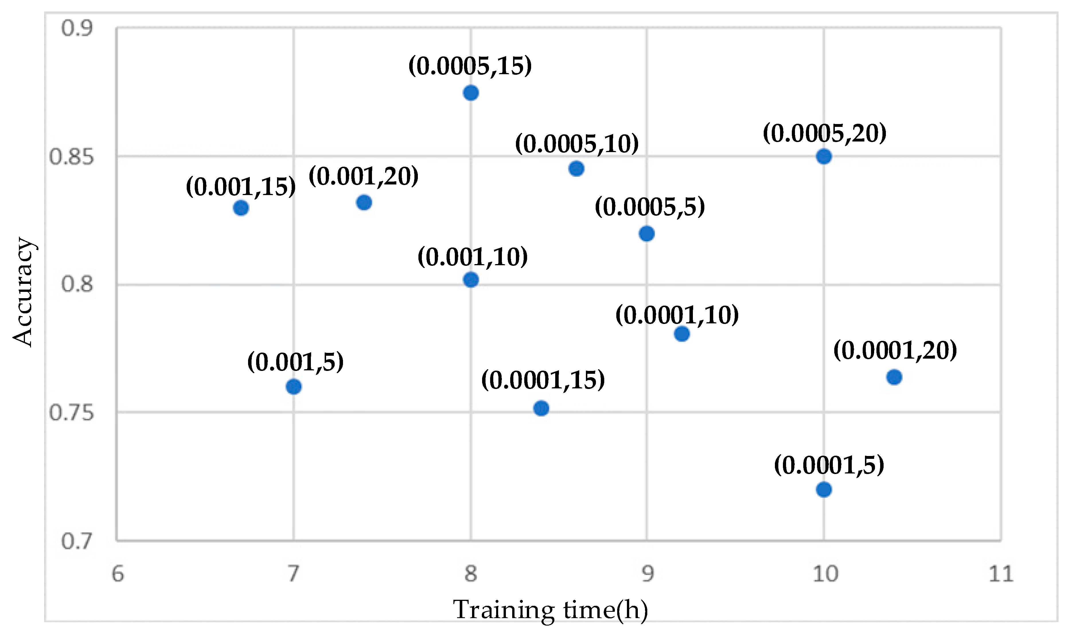
Experiment 2 tests the effects of different model parameters on the detection of overpasses. In Faster-RCNN, learning rate and batchsize are the two parameters that have the greatest impact on model results. Learning rate is a parameter that guides the model in adjusting the weight of the network through a loss function. The lower the learning rate, the slower the change in loss function. Batchsize is the number of samples used in one iteration. In a CNN, increasing the value of batchsize usually makes network converge faster, but due to the limitations of memory resources, if batchsize is too large, memory shortage will be insufficient, and the time consumed by the model to reach same accuracy will increase. Therefore, 12 sets of comparative experiments were performed using three different learning rates (0.0001, 0.0005, and 0.001) and four different batch sizes (5, 10, 15, and 20). The results of comparison experiment are shown in
Figure 11:
The results showed that when learning rate is 0.0005 and batchsize is 15, the model gives the best identification result. When the value of batchsize increases, the accuracy of the model does not changed substantially, and it takes too long to reach the same precision.
After training data was selected according to the method discussed in
Section 2.1, Experiment 3 compared the detection effect of training data with different geometric metrics. The results reflected the contribution of different geometric metrics to the identification of overpasses. The experiment results are shown in
Table 2.
The results showed that three geometric metrics (area, perimeter, rectangularity) have better performance on overpass identification, therefore, these adjusted geometric metrics are selected to synthetize the values of RGB bands in converted raster data.
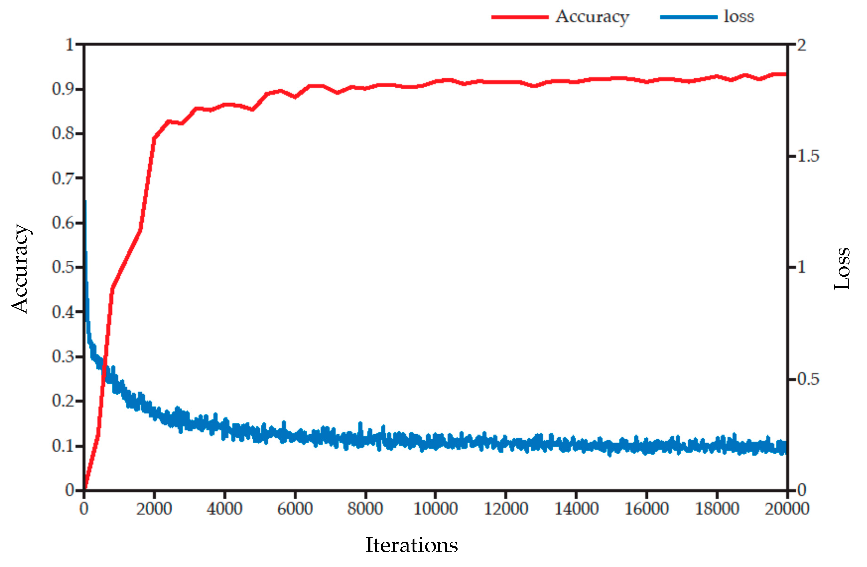
After the above comparative experiments, the optimized Faster-RCNN model was established and used to identify overpasses. The identification accuracy and the loss are shown in
Figure 12.
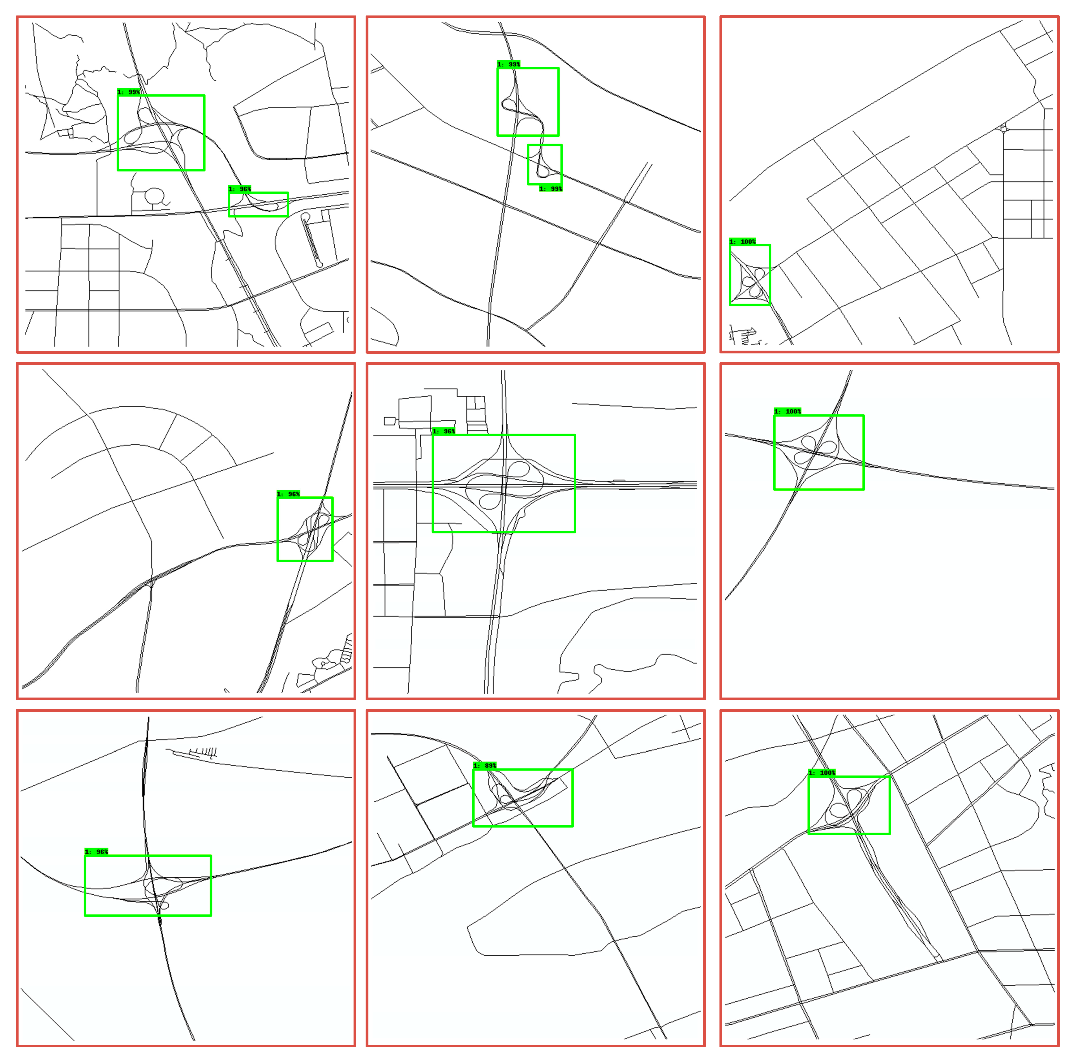
The identification results are shown in
Figure 13.
4. Conclusions
In this paper, Faster-RCNN was used to extract and learn the features of overpass structures in road networks and applied to overpass identification. The OLGDB was established to store labelled overpass data. The optimal model was obtained by evaluating the performances of various models with different geometric metrics-based training data, CNN structures, and training parameters. The accuracy of overpass identification reached up to more than 90%. The results showed that Faster-RCNN is effective for overpass identification. Faster-RCNN can learn the features of road networks well and can determine the position of overpasses in a complex road network with high accuracy. To the best of our knowledge, this study is the first attempt to identify overpasses using Faster-RCNN. Compared with traditional vector methods, this method does not require artificially designed features and avoids the uncertainty of experimental results caused by human intervention. The method performs well on actual road network data. In the future, we will expand the OLGDB, switch to more sophisticated target detection models, and attempt to identify other road network patterns under the deep learning framework. Also, we will continue to explore the applicability of this method in data of different scales or different urban road networks. And, besides OSM road data, we will discuss the impact of data from different sources on the identification results, such as road networks with more interfered road sections or road networks with missing parts of road sections.


