2. Entropies and Divergences—A Breviary
We consider a real valued random variable
x on a domain
. We denote by
a fixed probability density function (PDF); then,
and
. We fix a real valued differentiable function
, as a “controlling tool”. In this setting, the generalized (normalized) entropy is
We shall use a similar notation for other entropy-like functionals too. In the literature, the avatars of the “generalized logarithm” are subject to additional restrictions, imposed through applications inspired axioms.
Let
a smooth function and
an additional fixed PDF. We define
We suppose that and if and only if . The number is called the (generalized) divergence between and and measures to what extent influences . Sometimes, additional properties of the divergence function are added, axiomatically.
Example 1. With the previous notations, we recall some well-known examples of entropies ([35,36,37]). (i) In the particular case when , from Formula (1), we obtain the Boltzmann–Gibbs–Shannon (BGS) entropy. (ii) Consider a fixed parameter . The Tsallis q-logarithmprovides a Tsallis entropy. Usually, for , we use the notation . When , the BGS entropy is recovered. (iii) Let us fix . The Kaniadakis k-logarithmdefines a Kaniadakis entropy (named also k-deformed entropy). Usually, is denoted . When , we recover again the BGS entropy. (iv) Fix two real parameters k and r. The Sharma–Taneja–Mittal -logarithmprovides a Sharma–Taneja–Mittal (STM) entropy (also named -deformed entropy). Instead of , we shall denote . The Kaniadakis k- logarithm and the Tsallis q-logarithm are recovered as particular cases, for and for , respectively. When , we recover the BGS entropy. Sometimes, additional restrictions are imposed on the domain of the parameters, required by convergence conditions imposed on some integrals (see [38,39,40] for details). (v) ([27]) Let a positive, differentiable, strictly-increasing function. (Sometimes, in the literature, “non-decreasing” is required, instead of the “strictly-increasing” condition). Define the ϕ-deformed (Naudts) logarithm The function defines the ϕ-deformed (Naudts) entropy. The previous formula may also be read “backwards”: Moreover, given an arbitrary “generalized logarithm” φ as in (1), Formula (6) always provides a differentiable function ϕ; if it is positive and strictly-increasing, we expressed φ like a ϕ-deformed (Naudts) logarithm. Sometimes, this procedure works for some restrictions of the involved parameters only. For example, the preceding four entropies are recovered as particular cases of ϕ-deformed (Naudts) entropies, as follows: BGS for ; Tsallis for with the restrictions and ; Kaniadakis with the additional restrictionfor ; STM forwith the additional restrictionfor . These additional restrictions are imposed in order ϕ to be strictly-increasing. (vi) Let be a formal group logarithm, which is a differentiable real valued function with some special algebraic properties, inspired from the formal series linking Lie groups to Lie algebras. More precisely,where and . Its inverse iswhere , , , and so on. (We refer to [20,21,41] for details about these functions). The simplest example is . We define the generalized group entropy functional (GGEF) associated with (1) by In particular, for , we recover the well-known group entropy functional ([20,41]) associated with (1) Similar GGEFs can be provided by replacing the Neperian logarithm by other “generalized” logarithms (e.g., Tsallis, Kaniadakis, STM, etc). In Section 3, we shall introduce the geometries associated with the GGEF, based on ϕ-deformed (Naudts) entropies. Accordingly, we shall use the generalized logarithm from (5). Example 2. With the previous notations, we recall some well-known examples of divergences.
(i) An important particular case is the generalized (quotient) relative entropy (a.k.a. generalized divergence) between ρ and σ (see [34,42]) The function . We accept (formally) that , and . In particular, when , we recover the Kullback–Leibler divergence ([20]). Another particular case considers to be a convex function, with and . For , we recover the f-divergence ([43] and references therein). The slightly more general notion of -divergence (see [44]) may be recovered in a similar way. (ii) In a similar way, we define the generalized (difference) relative entropy between ρ and σ, as The function . In particular, when , coincides with D and we recover the Kullback–Leibler divergence, as in (i). When , the divergence D was considered in [27]; we mention that, in this case, does not coincide with D. In general, a necessary and sufficient condition on φ, ρ and σ, in order that , is the vanishing of the mean function . A sufficient (but quite strong) condition is provided by the functional equation .
(iii) In the hypothesis of Example 1 (vi), we can define generalized divergences as relative group entropies, which combine the formal group logarithm G, the φ-likelihood function and the previous quotient or difference operation upon two PDFs. For example, the analogue of (10) is (iv) Consider two fixed PDFs and . Denote as a fixed convex differentiable function. In this setting, the Bregman divergence is We mention that the function is convex too.
Let
be a
time-dependent PDF, where
. Then, the entropy in (
1) will also depend on the parameter
t, so
. We consider a
potential energy function and its associated
energy average function(If needed, restriction of these functions to open subsets is possible). This particular framework will be used in
Section 6 only.
3. Fisher-like Metrics Associated with Generalized Entropies and Generalized Divergences
In this section, we recall the notion of Fisher metric associated with a family of (generalized) entropies or divergences, defined on the space of parameters of an arbitrary PDF, using mainly [
20,
34]. For a more general setting, see [
34].
Consider the case when the PDF
in
Section 2 depends, moreover, on
n real parameters
, with
, where
is an open set of
. Thus,
,
. Let
be a differentiable controlling function,
. The dependence on
leads to a generalized entropy function
, canonically derived from Formula (
1):
In a similar natural way, we can define generalized divergence functions, by
-parameterizing (
2) and its avatars.
We suppose that the matrices
and
are non-degenerated, and
g has constant index on
. We call
g and
generalized Fisher metrics of type 1 and type 2, respectively, and denote GFM1 and GFM2. Both metrics are “means”, w.r.t.
, of some
-mediated “information matrices”: the Hessian of
and the matrix of the gradient of
with its transpose, respectively. The diagonal coefficients
,
, generalize the Fisher Information Numbers from [
45], which can be recovered when
is the Tsallis logarithm.
In general, the semi-Riemannian metric
g and the Riemannian metric
differ from each other and differ from the Hessian (semi-Riemannian metric if non-degenerated)
We define, in a formal way, two auxiliary symmetric tensors of (0,2)-type
and
, given by
and
We remark that, if non-degenerated, and provide semi-Riemannian metrics. In this case, these metrics are also of Fisher type, as they express “means” w.r.t. the PDF of two “derived information matrices”, of coefficients and , respectively.
Example 3. Consider the particular case of the BGS-entropy, with .
(i) In this case, both previous GFM1 and GFM2 coincide with the classical (Riemannian) Fisher metric associated with H (or φ) [20]. In the general case, it would be interesting to find all the controlling functions φ, for which g coincides with . Does this property necessarily imply that φ is proportional with , modulo a non-null constant? A further step would be to look for appropriate functions φ, in order that g and : be homothetic or conformal; have the same geodesics; have the same curvature, etc. To this differential geometric viewpoint, a statistical counterpart may eventually correspond.
(ii) Let be an open set and let , , …, , be smooth functions on X. Consider the PDF of exponential type, given by The associated Fischer metric is , which is a Hessian metric.
(iii) For this choice of the function φ, we obtain and , for . The “perturbed” Hessian matrix associated with α is similar to the one studied in some recent statistical applications (see, for example, [46]). Remark 1. (i) We give an interpretation and a motivation for the definition of the GFM1, in a slightly more general case than [20]. Consider φ a fixed controlling function. Let and be two families of parameterized PDFs over , with , and letbe the generalized (difference) relative entropy between them, as in (10). Denote and suppose its norm to be infinitesimally small. We know that has a unique minimum for , i.e., for . The Taylor decomposition around gives The second order approximation of this expression is precisely half of the GFM1 g, calculated in .
When , we recover the interpretation given in [20]. (ii) We do not know a similar interpretation for the GFM2 .
(iii) The generalized group relative divergences from Example 2 (iii) provide analogous formulas. We shall study them in the next section, in the particular case of the ϕ-deformed (Naudts) entropy.
(iv) The definition of Fisher metrics described previously is closely related to the need for understanding a variation of a PDF w.r.t. another (reference) one; the output of this “variational calculus factory” are functions. We signal here the forthcoming book [47], containing new revolutionary ideas in Variational calculus, including invariants of tensorial type, motivated by differential geometric problems; this source provides new insights for the definition and the study of divergence-like tensor fields, as a path toward a new bundle spaces approach in Statistics. (v) All the previous tensor fields g, , h, α, and β have constant index, one each connected component of their definition domains.
An open problem is to find the more general hypothesis such that these tensor fields be non-degenerated (in order to define semi-Riemannian metrics). Locally, the answer is simple: let be a point in the parameters space, such that the determinant of the corresponding matrix, calculated in , is not null. Then, the tensor field is non-degenerated in an open neighborhood of . For many families of examples (and in Section 5 we add several more ones), this property holds true. A common practice in the literature is to stop here, without investigating global conditions which are fulfilled in general cases. To our knowledge, global existence results for Fisher metrics, in the general setting, are not proven yet. Moreover, the eventual singular points have an interest in their own, as they may signal—in a suitable statistical model—a phase transition ([48]). We consider it useful to point out here the paper [49], where a different but correlated problem is studied: namely, to what extent the Fisher metric is (globally) unique, modulo the action of a diffeomorphism group. 4. The Fisher Geometries Associated with GGEFs Based on -Deformed (Naudts) Entropies and Divergences
We particularize now the results from
Section 3, for the case of the Naudts entropies. Let us fix the context more precisely.
Consider
a positive, differentiable and strictly-increasing function as in Example 1 (v) and the
-deformed (Naudts) logarithm
defined in Formula (
5). Let
,
be a family of parameterized PDFs, as in
Section 3. The associated GFM1
g and the GFM2
are obtained as particular cases from (
14) and (
15):
and
We suppose, as usual, that g and are non-degenerated and that has a constant index on X.
We also consider, via (
16), the associated Hessian metric
Proposition 1. With the previous notations, for every , we haveand In this case,
and
are given by
and
Corollary 1. In a condensed form, we have the following relation We consider now, in addition, a fixed formal group logarithm
G, as in Example 1 (vi). Let
be the associated parameterized PDFs and
be the generalized (difference) group relative entropy (a.k.a. the generalized (difference) group divergence), as particularization from (
10) and Remark 1 (i), (iii), written as
Denote the generalized group Fisher metric associated with
by
This Hessian-type metric will be calculated in the next result.
Proposition 2. With the previous notations, we have the relationwhich may be re-written as depending only on ϕ and ρ, in Proof. We follow the line of reasoning from [
20]. As
we calculate
Suppose, for the moment, that
is constant. Denote
We calculate successively
and
We replace
, and we use the property
. It follows that
From the last suite of formulas, we obtain both (
26) and (
27). □
Suppose, moreover, that
. Then, we have
We re-write this formula in a condensed form, and we obtain the following result, which completes Corollary 1.
Corollary 2. With the previous notations, for , we obtain By analogy, starting with a generalized (quotient) group relative entropy (a.k.a. the generalized (quotient) group divergence)
, as particularization from (
9), we shall obtain, in the sequel, other Fisher-like metrics, similar to the ones in Proposition 2 and Corollary 2.
Denote the generalized group Fisher metric associated with
by
Proposition 3. With the previous notations, we have the relationwhere denotes the classical Fisher metric. Proof. We adapt the proof of Proposition 2, from the divergence
to the divergence
. Suppose that
is constant. Denote
We assign
, and we use the property
. We obtain
The first integral equals
. The second integral is null because
. We obtained Formula (
30). □
Remark 2. (i) In Proposition 1, we establish the basic formulas for the future development of associated Riemannian geometries determined by g, , h, α, β, in terms of the function ϕ-deformed (Naudts) entropy (curvature, geodesics, Riemannian distance in the positive definite case). Examples of scalar curvature functions derived from these formulas will be shown in the next section. The coefficients of GFM1 g extend known ones from [29], derived for PDFs of exponential type and for particular functions ϕ. The other Fisher metrics are new. An interesting consequence of Proposition 1 is the fact that g and do not coincide, as in the case of the Neperian logarithm. This can be seen directly, by comparing their ϕ-dependent coefficients.
(ii) In Proposition 2, we derive the Fisher-like metric associated with the divergence , as a generalization of a construction in [30] for the case of a Kullback–Leibler divergence, of a trivial group logarithm and for PDFs of exponential type. (iii) In Proposition 3, the Fisher-like metric associated with the divergence is—to our knowledge—completely new.
The metrics in Formula (30) are homothetic, via a constant supposed—implicitly—to be not null. It is interesting that depends only on the behavior of the deformation function ϕ, for or around 1 and on G, around 0. Its independence on the PDFs gives an “universality” feature, which corresponds—probably—to some special uncovered property of the statistical model. Suppose, moreover, that . We replace in (30) the values and , and we obtain 5. Examples
We particularize now the results from
Section 4, for the case when
is an exponential PDF and
,
. The deforming function
will be chosen conveniently, in order to be able to compute the integrals.
Let
and
be the exponential (normal) PDF given by
We denote the partial derivatives of
, with respect to the variables
and
, by
,
,
,
,
. A short calculation ([
34]) leads to the formulas
The classical Fisher metric
has the coefficients
,
and
(see, for example, [
2,
34]).
For future calculations, we shall use the following simple result.
Lemma 1. Let c, , be fixed real constants, with , . Then, the semi-Riemannian metricon the set in has the scalar curvature In the sequel, we give examples of the semi-Riemannian metrics from Propositions 1–3, under various particular assumptions.
I—The case of g. Suppose
, with
an arbitrary fixed parameter. From Formula (
22), we calculate the coefficients
where
There exists a unique such that . For this value, g is degenerated. The metric g is Lorentzian, when and is Riemannian, when .
The scalar curvature
of
g is
The scalar curvature
does not vanish anywhere, and its sign is the opposite sign of
. Moreover,
is constant if and only if
, i.e., only in the case when
g is the classical Fisher metric
. If we decide to use the scalar curvature as a control, this may lead to a quick criterion to distinguish the BGS entropy case from the
-deformed (Naudts) entropy case. (The statistical interpretation of the scalar curvature of the Fisher metrics may be found in [
20]).
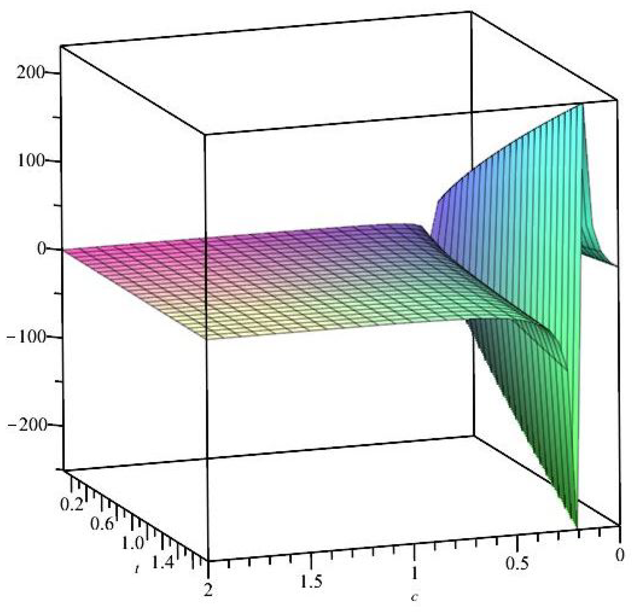
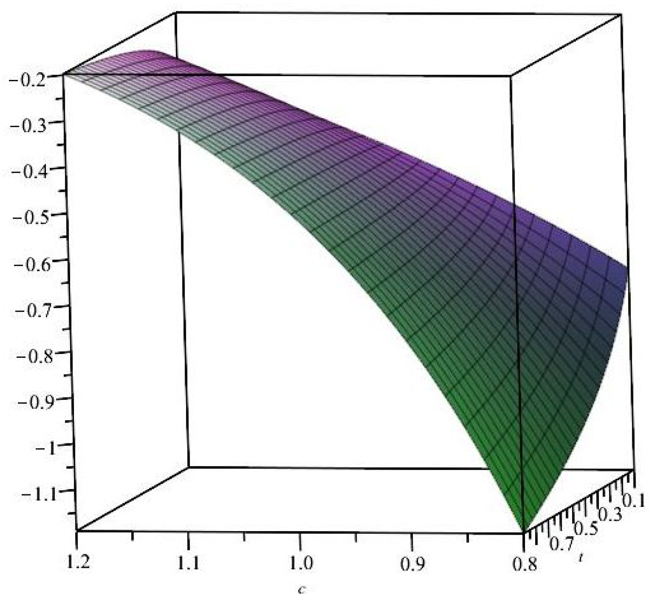
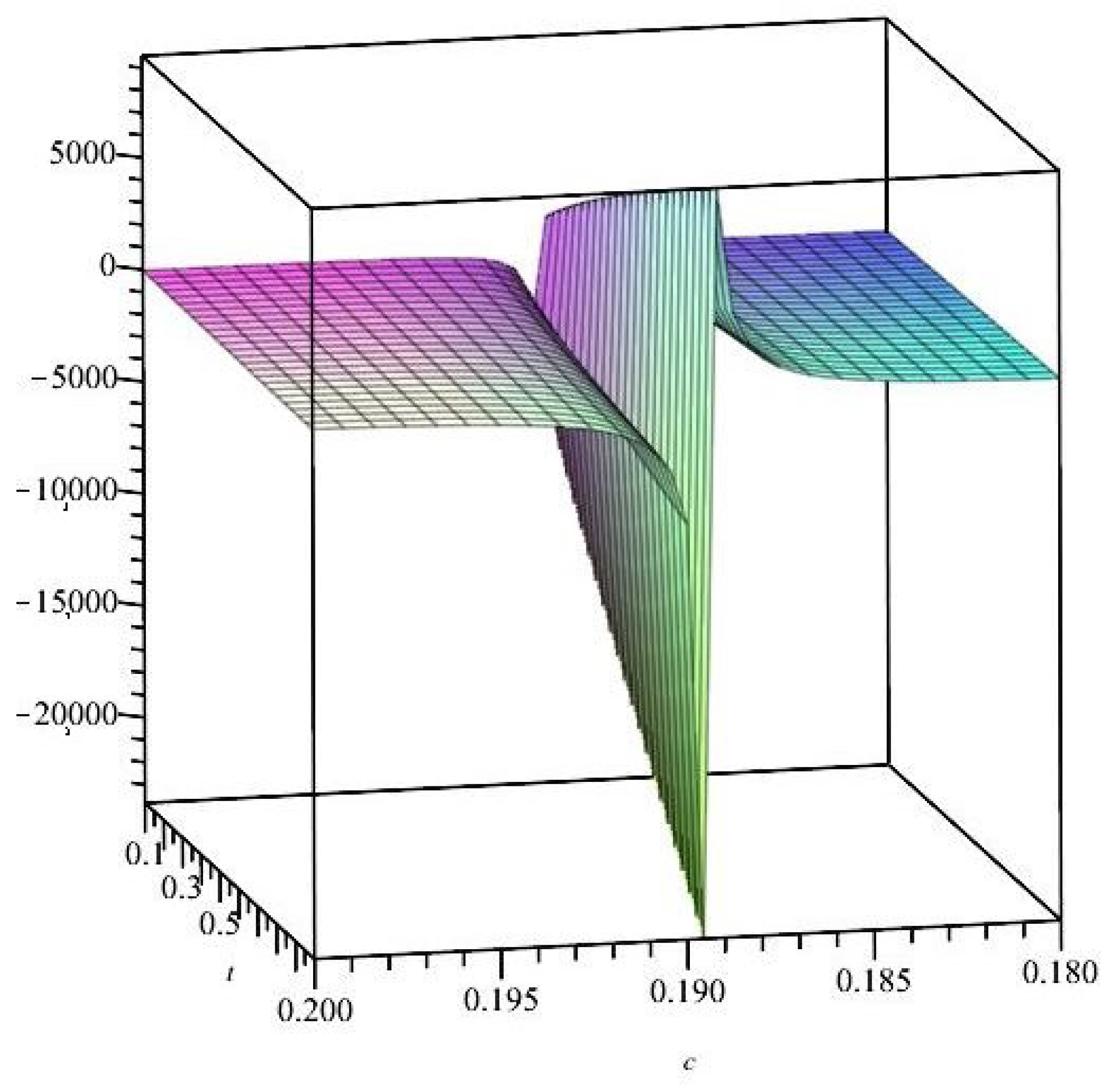
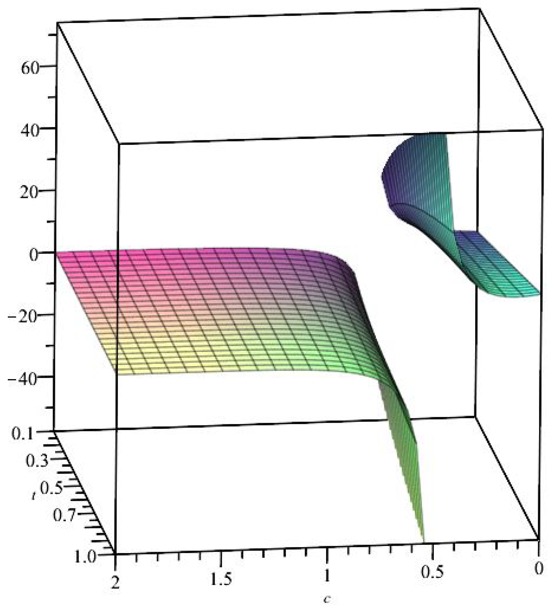
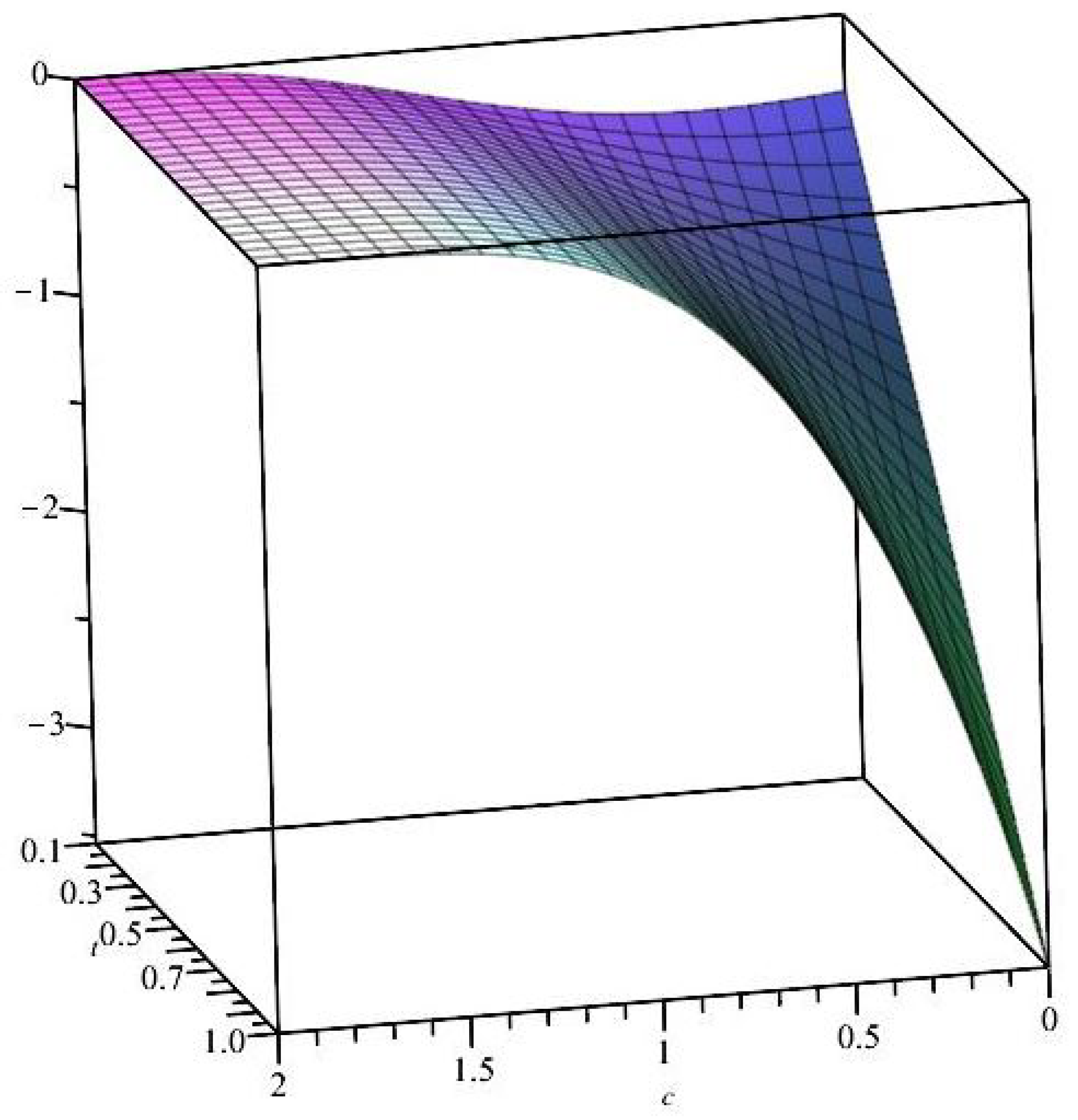
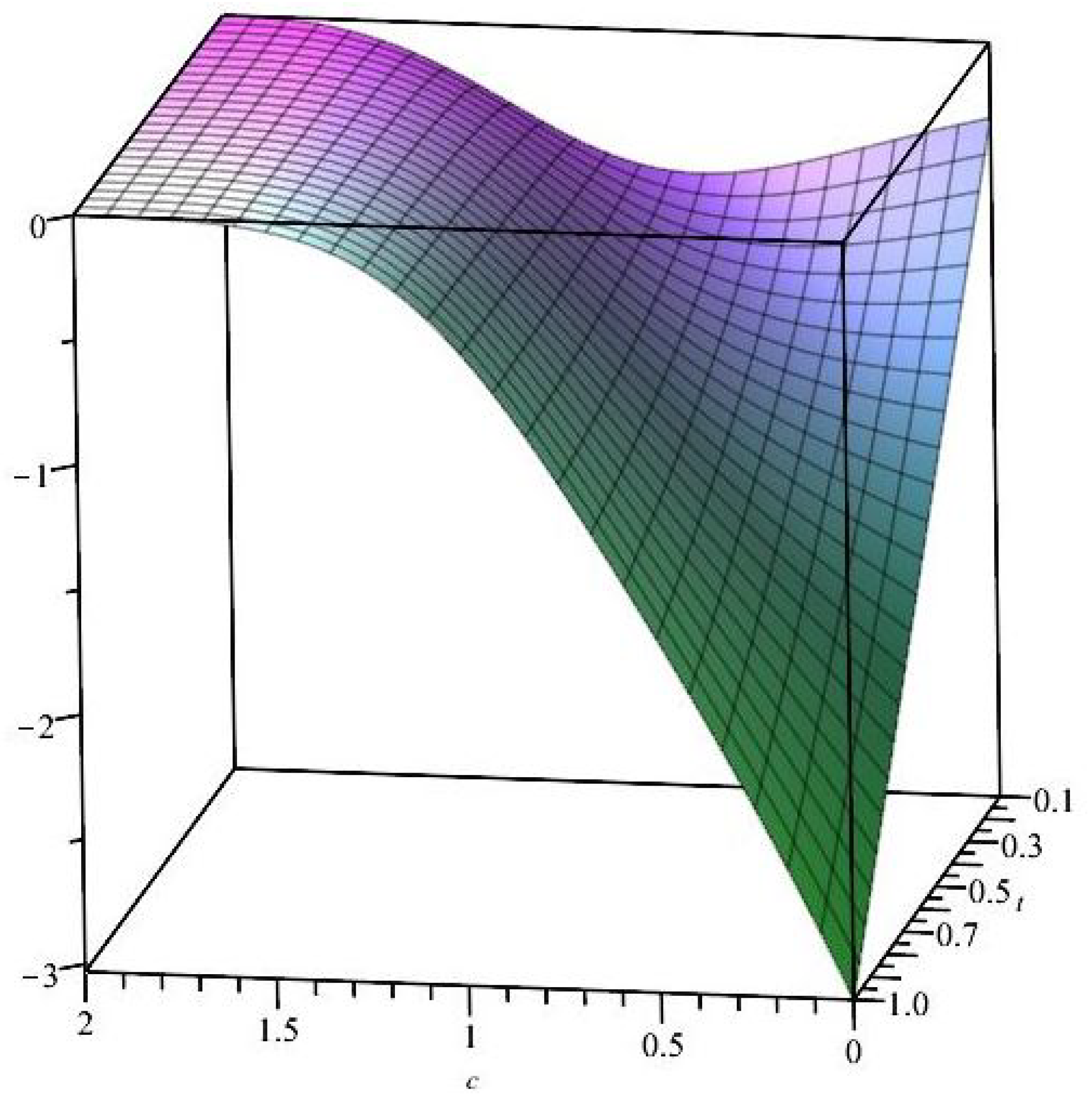
We depicted in
Figure 1 (and magnified in
Figure 2 around
and in
Figure 3 around
) how
varies w.r.t.
c and
(denoted
t).
II—The case of . Suppose
, with
an arbitrary fixed parameter. From Formula (
23), we calculate the coefficients
where
The scalar curvature
of the Riemannian metric
is
We mention that: the scalar curvature is negative; it decreases indefinitely as the variable
grows and the parameter
c goes to 0; it tends to 0 as
c goes to
. We depicted in
Figure 4 how
varies w.r.t.
c and
(denoted
t).
III—The case of h. Suppose
, with
an arbitrary fixed parameter. From Formula (
24), we calculate the coefficients
where
As the (0,2)-type tensor field h is degenerated, it does not define a semi-Riemannian metric. In this case, there is no scalar curvature to compute.
IV—The case of . Suppose
, with
an arbitrary fixed parameter. From Formula (
17) or from Proposition 1, we calculate the coefficients
where
The (0,2)-type tensor field is degenerated for . If , then is a Lorentzian metric. If , then is a Riemannian metric.
The scalar curvature
of
is
and has the sign of
. We depicted in
Figure 5 how
varies w.r.t.
c and
(denoted
t).
V—The case of . Suppose
, with
an arbitrary fixed parameter. From Formula (
18) or from Proposition 1, we calculate the coefficients
where
The scalar curvature
of
is
and takes negative values. We depicted in
Figure 6 how
varies w.r.t.
c and
(denoted
t).
VI—The case of . Suppose
, with
an arbitrary fixed parameter. From Formula (
27), we calculate the coefficients
where
We suppose that the group logarithm
G is chosen such that
be non-degenerated. The scalar curvature
of
is calculated using MAPLE:
Interestingly, the scalar curvature is a rational function of and .
We particularize now the setting for the BGS group logarithm
and replace
and
in the previous formulas. Then,
where
In this particular case, the scalar curvature
of the Riemannian metric
has the form:
(The same formula may be recovered, directly, by using Lemma 1.) We mention that
takes negative values, for every
. In
Figure 7, we depicted how this particular
varies w.r.t.
c and
(denoted
t).
VII—The case of . From (
30), we have the coefficients of
:
where
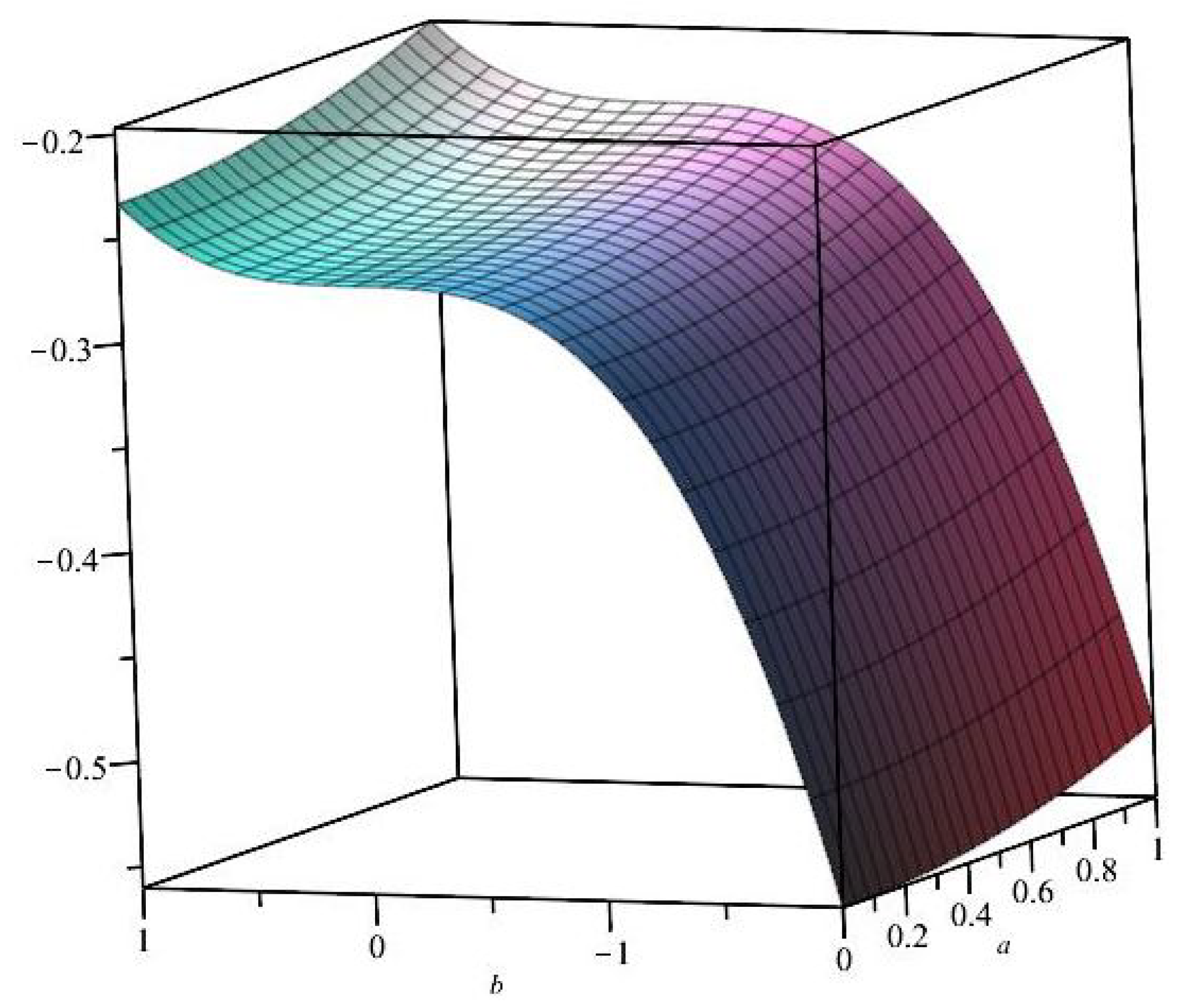
For the moment, we suppose that G and are suitable chosen, such that . It follows that is a Riemannian metric. As the scalar curvature of is a negative constant , we deduce the scalar curvature of is a negative constant w.r.t. too. In what follows, we study the variance of in two particular cases.
. Let
be the BGS grup logarithm function and consider
, where the real parameters
a and
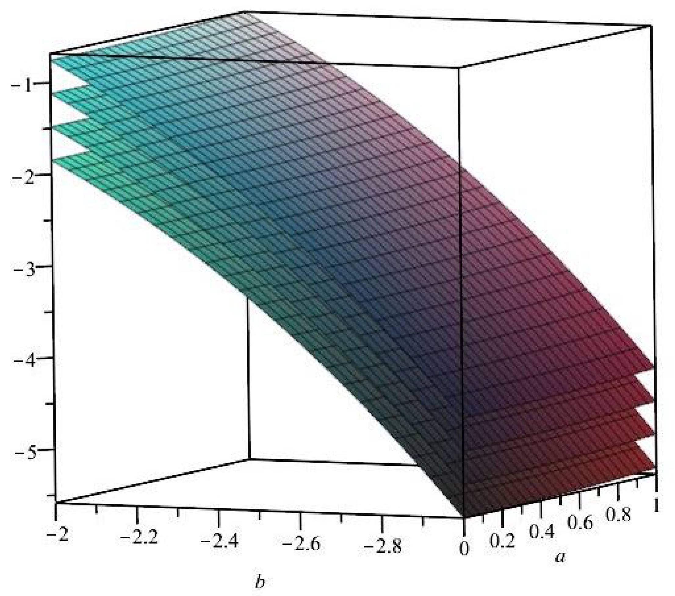
b satisfy
. Denote the respective metrics by
and their scalar curvatures by
. Then,
We mention that
(and hence
). The dependency of
w.r.t.
a and
b may be seen in
Figure 8.
The family of Fisher-like Riemannian metrics may be considered as evolving from the classical Fisher metric . Their evolution may be controlled through their scalar curvature.
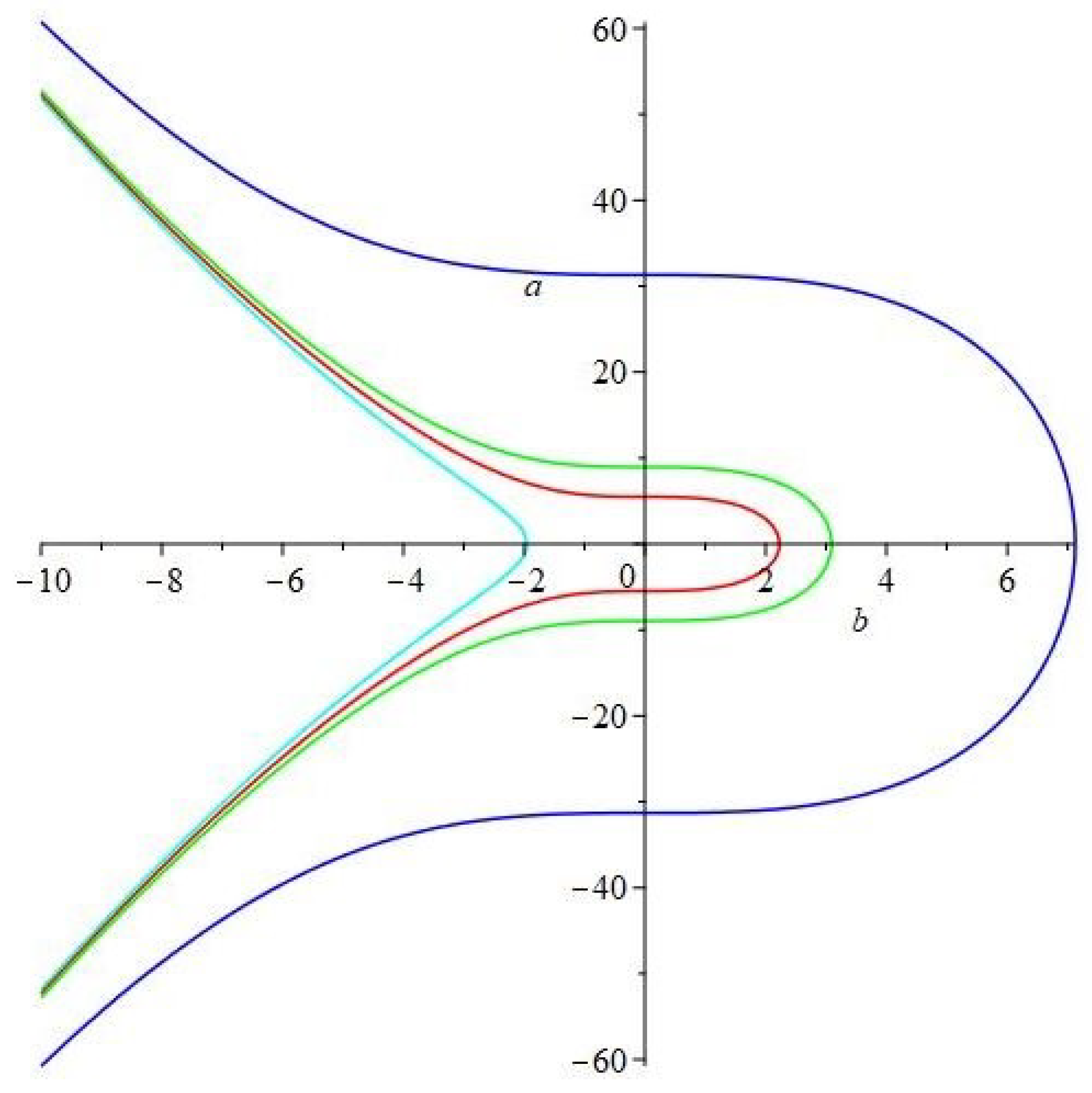
. Let
be the Tsallis grup logarithm function, where
. Let us define
, with real parameters
a and
b satisfying
. We denote the associated metric by
and its scalar curvature by
. Then,
We mention that
(and hence
). The dependency of
w.r.t.
a and
b may be seen in
Figure 9, for
q taking successively the values 1,11,21,31 (from bottom to top). The value
is no longer a forbidden (singular) one!
The family of Fisher-like Riemannian metrics may be considered as evolving from the classical Fisher metric , and also as “expanding” from the BGS group logarithm to the q-dependent Tsallis group logarithm. The evolution of these metrics may be controlled through their scalar curvature, which, in addition to the previous case , “foliates” following the values of q.
Remark 3. (i) The parameters’ domains are subsets of , which is two-dimensional. Therefore, for all the metrics in this section, the scalar curvature coincides with the Gaussian curvature. The coefficients of the metrics depend on the variable only, which has the signification of standard deviation. It follows that the scalar curvature functions are also independent on the mean of the PDF modeled by . This dependence of the geometric invariants only on the standard deviation suggests applications where a similar property appears: see, for example, [50,51,52,53,54]. (ii) Using general differential geometric arguments, we knew a priori that the metrics must be (locally) conformal with the Euclidean (or Minkowskian) metric of the plane. However, we obtained more: the conformal factors are explicitly derived, they are global and, as expected, they are also independent of the mean . Moreover, the metric in example is even homothetic with the Euclidean metric.
If we consider a curve in the parameters space, its length (w.r.t any of the respective metrics) depends only on the standard deviation; instead, the angle of two such curves does not depend on either the mean or the standard deviation.
(iii) The statistical significance of the sectional curvature of Fisher-like metrics g, , h, β, , can be obtained by analogy with Ruppeiner’s geometric modelization of the Gaussian thermodynamic fluctuations [55]. His “thermodynamic curvature” (R) corresponds to the sectional curvature and measures the inter-particles interaction: when , there is no interaction, and the cases or correspond to repulsive or attractive interactions, respectively ([55], apud [48,56]). This approach was developed and generalized by the Geometrothermodynamics theory [57]. Another viewpoint interprets the scalar curvature as a measure of the stability of the statistical model, in a direct proportionality relation ([58], apud [59]). (iv) It may be worth noting the following special property, apparently collateral to the main path of the discourse. Let us fix a value of the Tsallis parameter and a value of the scalar curvature in example , denoted by . Then, the solution of the equationis an elliptic curve in the plane of coordinates , written in Weierstrass form. In Figure 10, we drew these elliptic curves, corresponding to and to (from left to right). 7. Conclusions
(i) In this paper, we refined the search of relevant semi-Riemannian metrics associated in a canonical manner to manifolds of parameterized PDfs, via remarkable entropies and divergences. We stress the main general ideas:
- -
We made the distinction between quotient divergence and difference divergence, leading to different metrics
g and
(see Example 2 (i), (ii) and Formulas (
14) and (
15));
- -
We defined the (0,2)-type tensor fields
and
, as possible candidates for Fisher-like metrics (see (
17) and (
18));
- -
We gave an interpretation of the GFM1, whose coefficients may be derived from a variation of a generalized (difference) divergence (Remark 1 (i)).
(ii) In particular, based on the -deformed (Naudts) entropy, we focused on the following topics:
- -
We calculated the coefficients of the metrics g, , h, , , , in terms of and of the PDF (Propositions 1–3);
- -
When the PDFs are normal, univariate and depending on two parameters, we provided seven families of examples of the previous metrics; we determined formulas for their scalar curvature and we discussed its variation w.r.t. parameters;
- -
We proved a MaxEnt result (Theorem 1) for univariate PDFs and some extensions of the thermodynamic relations (Remark 4).
(iii) Future work will be directed toward:
- -
The search of the statistical relevance of and and a statistical interpretation for quotient divergences, similar to that for difference divergences (in the Remark 1 (i));
- -
The characterization of the case when the quotient divergence coincides with the difference divergence; this kind of result might bring into light unexpected—and eventually important—families of entropies;
- -
Refining the known families of deformation functions and finding new ones, relevant for applications. The interplay between the choice of and of the group logarithm G offers many modeling opportunities.
(iv) There exist two different but connected approaches to entropy: in Thermodynamics and in Statistical mechanics. Its geometrization by means of Fisher metrics follows two apparently different paths. The procedures to construct Fisher-like metrics from entropy are analogous, as they originate from the same general differential geometric methods. Instead, the basic manifold these metrics act upon (i.e., the space of the parameters) is essentially different. Moreover, entropy in Thermodynamics is “more deterministic” and one does not use a log-likelihood function which “produces” it.
The first formalism is dominated by the ideas of Weinhold, Ruppeiner and Quevedo [
55,
57,
63], and is extensively used in models for the entropy of black holes (see [
64] and references therein).
Our paper engaged in the second path and is dependent of log-likelihood functions, especially of the -deformed (Naudts) one. However, we are aware that more connections between the two theories are needed, with refined comparisons of the Riemannian models they both rely on.


 ,
, 


