A Combined Model-Order Reduction and Deep Learning Approach for Structural Health Monitoring under Varying Operational and Environmental Conditions ^†

Abstract

Nowadays, the aging, deterioration, and failure of civil structures are challenges of paramount importance, increasingly motivating the search of advanced Structural Health Monitoring (SHM) tools. In this work, we propose a SHM strategy for online structural damage detection and localization, combining Deep Learning (DL) and Model-Order Reduction (MOR). The developed data-based procedure is driven by the analysis of vibration and temperature recordings, shaped as multivariate time series and collected on the fly through pervasive sensor networks. Damage detection and localization are treated as a supervised classification task considering a finite number of predefined damage scenarios. During a preliminary offline phase, for each damage scenario, a collection of synthetic structural responses and temperature distributions, is numerically generated through a physics-based model. Several loading and thermal conditions are considered, thanks to a suitable parametrization of the problem, which controls the dependency of the model on operational and environmental conditions. Because of the huge amount of model evaluations, MOR techniques are employed in order to relieve the computational burden that is associated to the dataset construction. Finally, a deep neural network, featuring a stack of convolutional layers, is trained by assimilating both vibrational and thermal data. During the online phase, the trained DL network processes new incoming recordings in order to classify the actual state of the structure, thus providing information regarding the presence and localization of the damage, if any. Numerical performances of the proposed approach are assessed on the monitoring of a two-storey frame under low intensity seismic excitation.

1. Introduction

Modern societies are strongly dependent on the use of complex structures. Because an early detection of structural faults can greatly reduce the maintenance cost over time and prevent catastrophic events [1], being able to keep civil constructions safe and reliable is fundamental for community welfare [2]. For these reasons, in the last decades, civil engineering has focused on Structural Health Monitoring (SHM) [3], which aims at detecting, localizing, and quantifying damage occurrence. Especially, data-driven approaches [4,5] are becoming increasingly widespread thanks to their capacity of easily manage the large amount of data, acquired through pervasive sensor networks. In particular, by processing raw vibrational signals (e.g., acceleration recordings that are shaped as multivariate time series), they can extract useful features, in order to determine the damage state of the structure. To this aim, Deep Learning (DL) algorithms can automatically extract damage-sensitive features [6] and relate them with the corresponding structural states, by exploiting temporal correlations within and across time recordings.

When considering a finite number of predefined damage scenarios, the detection and localization of damage in structures can be treated within a classification framework. By employing a supervised classifier, the goal is to predict the categorical class (i.e., a label referring to a predefined damage scenario) of new incoming data, on the basis of past observations. Supervised techniques require labeled data on the possible damage conditions of the structure, which, however, are hard (if not impossible) to acquire for civil applications. This drawback calls for a Simulation-Based Classification (SBC) [1,7,8], in order to numerically simulate the effect of damage on the structural response. In such hybrid model-data SHM approach, a dataset of synthetic time-signals, accounting for relevant operational conditions and varying environmental effects, is generated through simulations of a physics-based model, for the whole set of considered damage scenarios and, thus, assimilated with the DL algorithm.

In order to replace the expensive numerical models, relying on the Finite Element (FE) method, a Model Order Reduction (MOR) strategy, such as the Reduced Basis (RB) method [9,10], can be adopted in order to accelerate the dataset construction.

The proposed methodology exploits an offline-online decomposition. During the preliminary offline phase, our DL-based classifier is trained on a numerically pre-built dataset of labeled inputs; during the online phase, the trained classifier processes unseen experimental signals that were acquired on the fly, returning, as output, the structural state that might have most likely produced them. Our classifier is based on a Fully Convolutional Network (FCN) architecture, which was already successfully applied in [8,9].

Additional to damage phenomena, environmental conditions could affect measured signals. Thermal fluctuations (both daily and seasonal) can influence a wide range of material properties and induce structural displacements. It is not easy to distinguish these effects from those of damage. For this reason, the thermal effects are simulated in the numerical model of the structure and temperature measurements are used together with vibrational ones as inputs to the classifier.

2. SHM Methodology: Dataset Definition and Damage Classifier

Considering an observation windows $(0,T)$, short enough to assume frozen operational, environmental, and damage conditions, the damage state of the structure is monitored by collecting vibrational and temperature data through a sensor network featuring $N_u$ vibrational sensors, with a fixed sampling period $\Delta t$, and $N_{\varphi }$ thermometers. The network arrangement has been designed starting from an initial placement involving a high number of sensors, progressively reduced evaluating the classifier performances on multiple datasets that were generated according to different sensor configurations. Vibrational recordings consist of displacement and/or acceleration measurements ${\mathbf{u}}_n,{\ddot{\mathbf{u}}}_n$ ($n=1,\dots ,N_u$) of length $L=T/\Delta t$ (for the sake of simplicity, in this section we only consider displacement measurements), while each thermometer outputs a single value ${\varphi }_n$$(n=1,\cdots ,N_{\varphi })$. A single data instance is composed of a set of displacement recordings ${\mathbf{U}}_i({\mathit{\eta }}_u^i,{\mathit{\eta }}_{\varphi }^i,g_i)=[{\mathbf{u}}_1^i,\dots ,{\mathbf{u}}_{N_u}^i]\in {\mathbb{R}}^{L\times N_u}$ and temperature measurements ${\mathbf{\Phi }}_i\left({\mathit{\eta }}_{\varphi }^i\right)=({\varphi }_1^i,\dots ,{\varphi }_{N_{\varphi }}^i)\in {\mathbb{R}}^{N_{\varphi }}$, where: $g_i$ labels the damage state that is undergone by the structure in the i-th instances, modeled as a localized stiffness reduction in pre-designated regions; ${\mathit{\eta }}_u^i$ and ${\mathit{\eta }}_{\varphi }^i$ label the set of parameters that control the mechanical and the temperature field, respectively. The dataset $\mathbf{D}$ is made of I instances $\{{\mathbf{U}}_i,{\mathbf{\Phi }}_i\}$, $i=1,\cdots ,I$; to relieve the computational burden of its generation, the Full-Order Model (FOM), which relies on the FE method, is replaced by a Reduced-Order Model (ROM).

According to the adopted classification framework, only a discrete number of damage scenarios $g=0,\dots ,G$ has to be defined on the basis of the mechanical behavior, load conditions, and aging processes interesting similar structures [4]. The baseline undamaged state is labeled as $g=0$.

A continuous probability density function (pdf) describes the occurrence of each entry of ${\mathit{\eta }}_u^i$ and ${\mathit{\eta }}_{\varphi }^i$, while a discrete pdf governs the occurrence of $g_i$. The parameter set ${\mathit{\eta }}_{\varphi }^i$, which is sampled from pdfs that take the locality of interest and the seasonality of temperature fluctuations into account, controls the temperature profiles that are imposed at the domain edges. The set ${\mathit{\eta }}_u^i$ parametrizes the external loads (e.g., amplitude and frequency of a dynamical load) and the damage level ${\delta }_i$, intended as the intensity of the stiffness reduction involving the subdomain that is related to $g_i$. A suitable sampling rule (e.g., a Latin Hypercube Sampling) has been adopted in order to explore the parametric space defined combining ${\mathit{\eta }}_u$, ${\mathit{\eta }}_{\varphi }$ and g. Each sampling ${\{{\mathit{\eta }}_u,{\mathit{\eta }}_{\varphi },g\}}_i$ uniquely identifies the corresponding dataset instance $\{{\mathbf{U}}_i,{\mathbf{\Phi }}_i\}$.

Once built, $\mathbf{D}$ is employed to train and validate a classifier $\mathcal{G}$. During the training phase, $I_{tr}$ instances are employed by $\mathcal{G}$ to learn the underlying mapping between the i-th instance $\{{\mathbf{U}}_i,{\mathbf{\Phi }}_i\}$ and $g_i$, while $I_{val}$ instances (with $I=I_{tr}+I_{val}$) are used in order to validate the learning process. Once trained, $\mathcal{G}$ should be able to correctly map an unseen instance $\{{\mathbf{U}}_i,{\mathbf{\Phi }}_i\}$ into the correct damage state $g_i$. In the absence of experimental data, the generalization capabilities have been assessed on a test set built through FOM simulations, in this way ensuring better fidelity to the experimental framework. For sake of clarity, from now on, we disregard specifying the instance index i.

Our FCN architecture, resembling the one that is proposed in [8], processes $\mathbf{U}$ by exploiting a stack of three Convolutional Units (CU), followed by a Global Average Pooling (GAP), whose output is merged with $\mathbf{\Phi }$ through a Concatenation Block (CB). These latter support the classifier in recognizing thermal effects of material contraction/expansion and stiffening/softening within the observed dynamics, in order to not confuse the environmental variability with damage [11]. Thus, a dense layer operates a linear mapping, ruled by a weight matrix $\mathsf{\Theta }$, allowing a final Softmax layer to perform the classification task. Each of the three CUs is formed by a Convolutional Layer (CL), together with Batch Normalization, in order to stem gradient instability issues during training, and ReLU activation function. In a CL, connection weights $\mathsf{\Omega }$ can be imagined as filters of kernel size $H_j$, with $j=1,2,3$, to be applied to the output of the previous layer. Each convolutional layer applies $N_j$ filters to its inputs, yielding an output that is made of $N_j$ feature maps. This composition of nonlinear transformations makes each damage target class linearly separable and allows for addressing the temporal pattern recognition, exploiting inter-sensor correlations, by simultaneously analyzing $\mathbf{U}$. The GAP condenses the resulting feature maps, which elicits a single, yet highly informative, description of its input channel ${\mathbf{u}}_1,\dots ,{\mathbf{u}}_{N_u}$.

While training $\mathcal{G}$, the learning algorithm tunes the weights $\mathsf{\Omega }$ and $\mathsf{\Theta }$, by iteratively minimizing a loss function over the $I_{tr}$ instances. The adopted loss function is the cross entropy, as is usually done in classification frameworks; Adam, a first-order stochastic gradient descend algorithm, has been employed in order to perform the iterative minimization process. At each iteration, a certain number of instances B, called mini-batch, are simultaneously analyzed in order to update the connection weights; each time all of the $I_{tr}$ instances have been processed is said to be an epoch.

The FCN hyperparameters ($N_j,H_j,B,I,{\mathrm{n}}^{\circ }\mathrm{epochs}$), initially set according to [8], have been tuned through the repeated evaluation of the classification accuracy. Herein, we have adopted: $N_1=16$, $N_2=32$, and $N_3=16$, as the number of filters; $H_1=8$, $H_2=5$ and $H_3=3$, as kernel sizes; $B=16$ as mini-batch size; $I=15000$, as number of instances, with the ratio $I_{tr}:I_{val}=75:25$; 1000 training epochs.

3. SHM Methodology: Dataset Population

Adopting a SBC approach, the generation of the I instances has been carried out by evaluating the physics-based model of the structure, for multiple values of the input parameters ${\mathit{\eta }}_u$ and ${\mathit{\eta }}_{\varphi }$ for each considered scenario $g=0,\cdots ,G$.

The thermo-mechanical behavior of the structure has been modeled through the standard linear thermo-elasticity theory employing a one-way coupling approach; the thermal field is independently determined from the kinematic one, but it still influences the material deformations. Moreover, having supposed monitoring windows of fixed duration, being significantly lower than the time that is required to experience notable temperature excursions, the thermal field has been evaluated while disregarding its temporal dependence. In order to reflect an oscillation of the material temperature into the dynamical response, a local dependency of the Young modulus E on temperature has been introduced. Lastly, damping effects have been disregarded due to the small relevance in the identification of continuously excited dynamic systems [12,13]; besides, modeling the structural damage as a selective reduction in stiffness, frozen in $(0,T)$, the mechanical behavior has been treated as linear [3]. The FOM reads, as follows:

$${\mathbf{K}}_{\phi }\mathit{\phi }={\mathbf{f}}_{\phi },$$

(1)

$$\left\{\begin{array}{c}{\mathbf{M}}_v\ddot{\mathbf{v}}\left(t\right)+{\mathbf{K}}_v\mathbf{v}\left(t\right)={\mathbf{G}}_v\mathit{\phi }+{\mathbf{f}}_v\left(t\right),t\in (0,T)\hfill \\ \mathbf{v}\left(0\right)={\mathbf{v}}_0\hfill \\ \dot{\mathbf{v}}\left(0\right)={\dot{\mathbf{v}}}_0\hfill \end{array}\right.,$$

(2)

and results from a Galerkin–FE discretization of a stationary diffusion problem and of a elasto-dynamic problem with a coupling term, respectively. In particular: $t\in (0,T)$ denotes the time coordinate; $\mathit{\phi }=\mathit{\phi }\left({\mathit{\eta }}_{\varphi }\right)\in {\mathbb{R}}^{M_{\phi }}$ is the temperature vector; ${\mathbf{K}}_{\phi }\in {\mathbb{R}}^{M_{\phi }\times M_{\phi }}$ is the thermal conductivity matrix; ${\mathbf{f}}_{\phi }={\mathbf{f}}_{\phi }\left({\mathit{\eta }}_{\varphi }\right)\in {\mathbb{R}}^{M_{\phi }}$ is the thermal right hand side vector; $\mathbf{v}=\mathbf{v}(t,{\mathit{\eta }}_u,\mathit{\phi },g)\in {\mathbb{R}}^{M_v}$ is the displacement vector; ${\mathbf{M}}_v\in {\mathbb{R}}^{M_v\times M_v}$ is the mass matrix; ${\mathbf{K}}_v={\mathbf{K}}_v(\mathit{\phi },g)\in {\mathbb{R}}^{M_v\times M_v}$ is the elastic stiffness matrix; ${\mathbf{G}}_v\in {\mathbb{R}}^{M_v\times M_{\phi }}$ is the coupling term; ${\mathbf{f}}_v={\mathbf{f}}_v(t,{\mathit{\eta }}_u)\in {\mathbb{R}}^{M_v}$ is the mechanical right hand side vector; $M_{\phi }$ and $M_v$ denote, respectively, the number of degrees of freedom (dofs) of the temperature and the displacement FE spaces.

Pb. (1) is first solved in order to determine the temperature field $\mathit{\phi }$. Vector $\mathit{\phi }$ is transformed into equivalent nodal forces through ${\mathbf{G}}_v$. A displacement field, compatible with $\mathit{\phi }$, is determined by solving a static mechanical problem under the coupling action only, and it is assumed as the reference around which the dynamics that are governed by Pb. (2) oscillates. Discretization in time has been made according to the sensors sampling rate. For the integration in time of Pb. (2), we have exploited a generalized-$\alpha$ method.

The FOM relies upon a number of dofs $M_v$ and $M_{\phi }$, depending on the adopted (potentially fine) discretization. The RB method, which is used to construct the dataset $\mathbf{D}$, exploits a Galerkin-Proper Orthogonal Decomposition (POD) ROM, whose POD basis is built, starting from a set of FOM solutions (snapshots), which are computed within the prescribed parameters range. The ROM solution is then sought by solving the reduced-order problem resulting from the Galerkin projection of the FOM onto the reduced basis.

Displacements and temperatures that are related to the i-th sampling $\{{\mathit{\eta }}_u,{\mathit{\eta }}_{\varphi },g\}$ are time integrated and collected in $\mathbf{V}=[{\mathbf{v}}_1,\dots ,{\mathbf{v}}_L]\in {\mathbb{R}}^{M_v\times L}$ and $\mathit{\phi }={({\phi }_1,\dots ,{\phi }_{M_{\phi }})}^{\top }\in {\mathbb{R}}^{M_{\phi }}$, respectively. The monitored dofs $\mathbf{U}$ and $\mathbf{\Phi }$, mimicking the sensors recordings, are extracted through two boolean matrices ${\mathbf{T}}_u\in {\mathbb{R}}^{N_u\times M_v}$ and ${\mathbf{T}}_{\varphi }\in {\mathbb{R}}^{N_{\varphi }\times M_{\phi }}$, as $\mathbf{U}={\left({\mathbf{T}}_u\mathbf{V}\right)}^{\top }$ and $\mathbf{\Phi }={\left({\mathbf{T}}_{\varphi }\phi \right)}^{\top }$.

4. Numerical Test Case

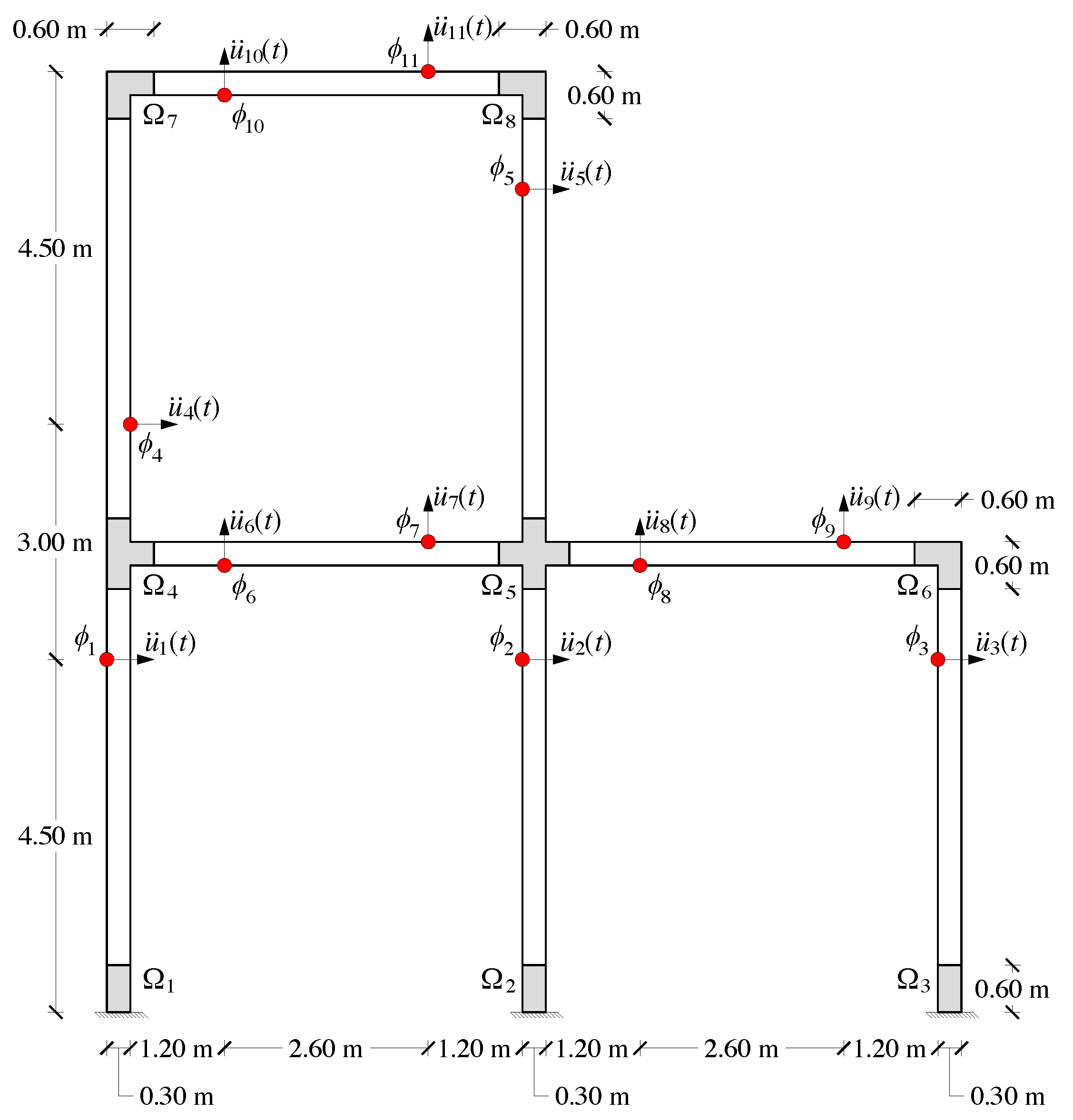
The proposed approach has been assessed on the monitoring of the two-dimensional (2D) frame that is depicted in Figure 1. When considering a structural thickness of $0.1$ m, the plane stresses formulation has been adopted. The bottom edges are assumed perfectly clamped to the ground. The geometry has been discretized in 2938 constant strain triangle finite elements. The adopted mechanical and thermal properties are those of an ordinary reinforced concrete: Young modulus $E=30$ GPa; Poisson ratio $\nu =0.2$; density $\rho$ = 2500 kg/m${}^3$; thermal expansion coefficient ${\alpha }_L=12·{10}^{-6}{}^{\circ }$C${}^{-1}$; stiffness thermal coefficient ${\alpha }_E=4.5·{10}^{-4}{}^{\circ }$C${}^{-1}$. The last two proprieties allow for relating the local material temperature to the thermally induced anelastic deformations and the material stiffening/softening, respectively.

The structure is excited by low intensity seismic loads. To this aim, we have employed the empirical equations for predicting the attenuation of ground motion proposed in [14] and implemented in [15]. The main advantage of this tool is the possibility to generate random spectrum-compatible accelerograms as a function of: local magnitude Q; epicentral distance R; and, site geology. In order to ensure the structure to behave in elastic regime, those parameters have been limited within the following ranges: $Q\in (4.8,5.3)$; $R\in (80,100)$ km; rocky conditions. The parameters Q and R have been described by two uniform pdfs ${\mathcal{U}}_Q(4.8,5.3)$ and ${\mathcal{U}}_R(80\mathrm{km},100\mathrm{km})$, respectively.

Nine damage scenarios have been simulated by means of a localized stiffness reduction. Each structural state $g\in \{1,\cdots ,8\}$ identifies a structural damage that occurs in the subdomain ${\mathsf{\Omega }}_s$, $s=1\cdots ,8$, respectively; the damage-free baseline is labeled as $g=0$. The occurrence of damage scenarios has been modeled with a (discrete) uniform pdf ${\mathcal{U}}_g\left(\{0,\cdots ,8\}\right)$ describing g. The damage level $\delta$, which represents the intensity of the stiffness reduction to be applied, has been modeled by a uniform pdf ${\mathcal{U}}_{\delta }(5\%,25\%)$.

In order to simulate potential thermal distributions, resembling those that are experienced by the structure, Pb. (1) is solved under the action of thermal profiles that are imposed on all edges. Those profiles have been modeled by interpolating temperature values at edges midpoints and corners, which are nothing but the components of the parameter vector ${\mathit{\eta }}_{\varphi }$. Temperatures have been assumed to be constant and equal for the three edges in contact with the ground, while parabolic profiles have been used elsewhere. In this way, a total of 28 parameters ${\mathit{\eta }}_{\varphi }^l$ (with $l=1,\cdots ,28$) are involved. From the temperature data of the city of Milan, a Gaussian pdf ${\mathcal{N}}_m({\mu }_m,{\sigma }_m)$, $m=1,\cdots ,12$, has been defined for each month, with ${\mu }_m$ and ${\sigma }_m$ being the monthly average and standard deviation, respectively. Each time Pb. (1) is solved, the month occurrence is sampled from a (discrete) pdf ${\mathcal{U}}_m\left(\{1,\cdots ,12\}\right)$, thus the ${\mathit{\eta }}_{\varphi }^l$ are inferred from the corresponding pdf ${\mathcal{N}}_m({\mu }_m,{\sigma }_m)$.

The sensor network consists of $N_u=11$ sensors, recording structural accelerations ${\ddot{u}}_n\left(t\right)$, and of $N_{\varphi }=11$ thermometers, recording temperatures ${\varphi }_n$, with $n=1,\cdots ,11$, being arranged as depicted in Figure 1. We have considered dual output sensors, recording both accelerations and temperatures at the same location. The dynamical response is monitored with a sampling frequency of 20 Hz, so as to sample the first two structural frequencies, respectively, 2.79 Hz and 7.14 Hz, without incurring in aliasing.

Thanks to the adoption of the ROM for the dataset construction, the number of dofs decreases from $M_{\phi }=1469$ to 28 for the stationary diffusion problem and from $M_v=2938$ to 63 for the elasto-dynamic problem. Consequently, the CPU time that is required by each simulation, over the time interval $(0,T=35\mathrm{s})$, passes from 421 s to $4.9$ s, entailing a speed-up of about 86 times (computations have been run on a PC featuring an Intel (R) Core™, i5 CPU @ 2.6 GHz and 8 GB RAM).

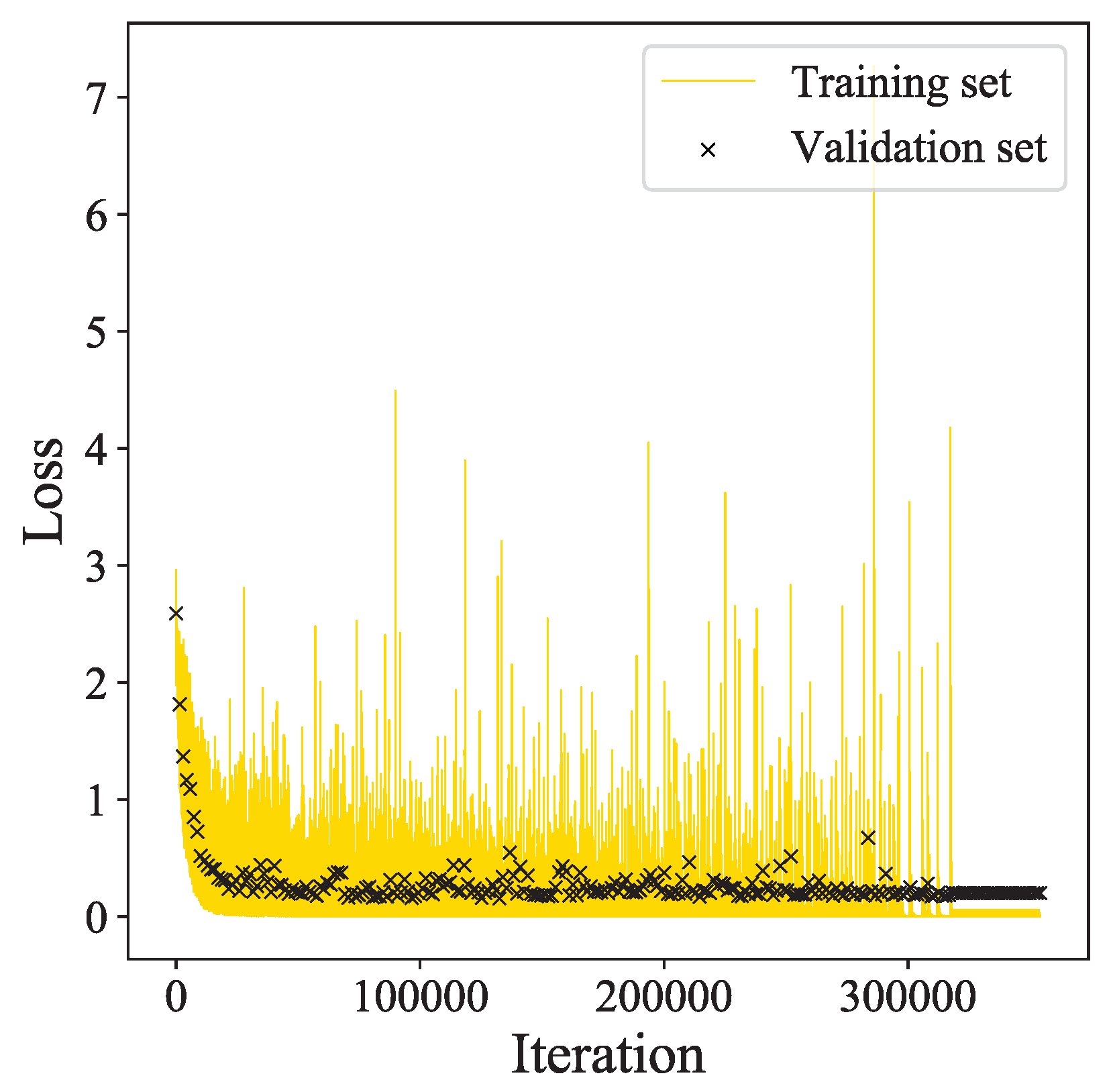
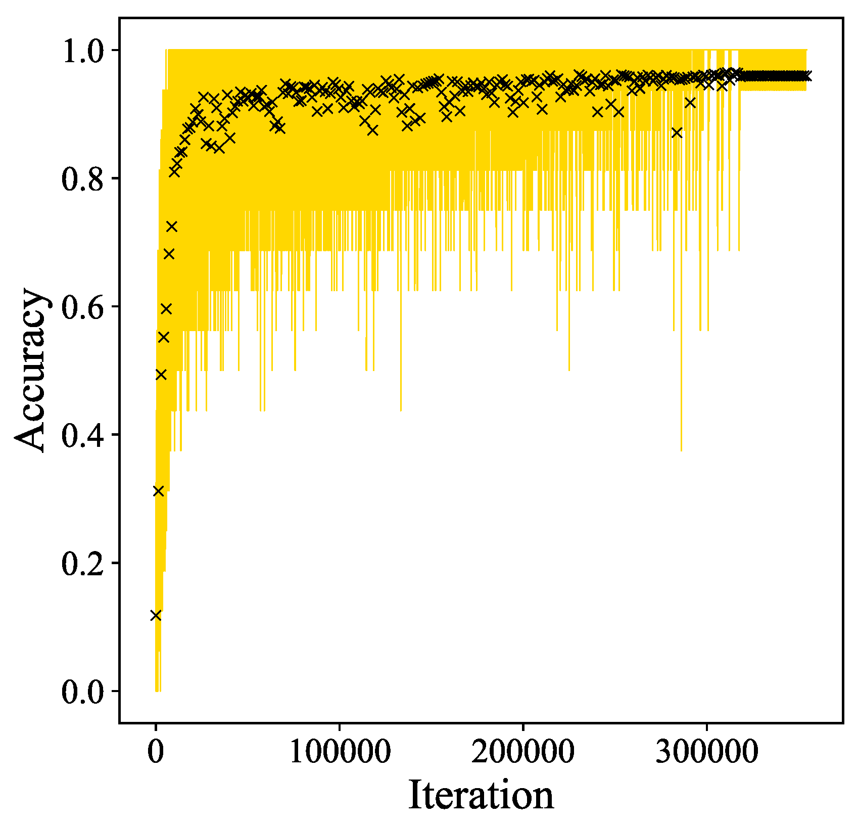
The evolution of the loss function and global accuracy of classifier $\mathcal{G}$, obtained during the training, are respectively reported in Figure 2 and Figure 3. The iteration number accounts for the number of times the FCN weights have been updated. The greatest gains in terms of classification accuracy (i.e., the ratio of correctly classified instances over the total) are obtained in the first portion of the graph.

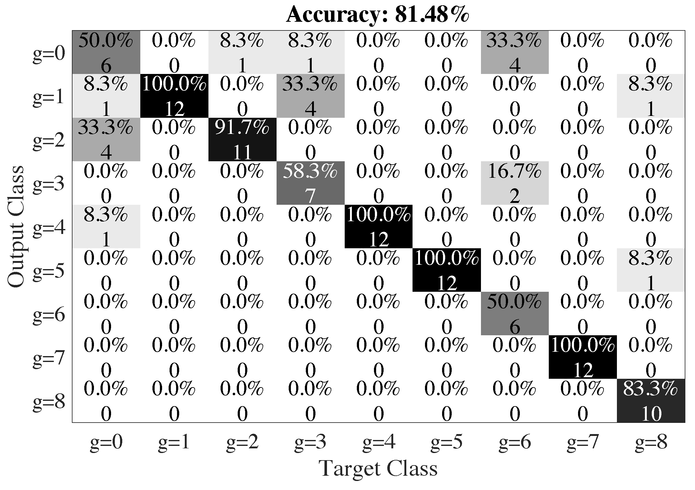
The generalization capabilities of the classifier $\mathcal{G}$ have been assessed on a test set made of 108 pseudo-experimental instances that are generated through the FOM. The classifier $\mathcal{G}$ carries out the classification task with a global accuracy of $81.48\%$ and a testing time of $1.08$ s, which means roughly about $0.01$ s for each test instance. The obtained results are summarized by the confusion matrix in Figure 4. Two different sources of error stand out. In particular, a small number of test instances labeled as $g=3$ are misclassified as $g=1$ (the same also occurs between $g=6$ and $g=3$); this might be due to the similar influence of those scenarios on the mechanical behavior. Moreover, half of the test instances that are labeled as $g=0$ (undamaged) are also misclassified; this might be due to the variability of $\delta$. Indeed, a low value of $\delta$ not only implies an augmented difficulty in distinguishing between damaged and undamaged conditions, but it also causes the ROM to be less accurate.

5. Conclusions

In this work, we have proposed a computational framework, integrating model-order reduction and deep learning, for structural health monitoring under varying operational and environmental conditions. This hybrid model-data strategy enables online damage localization, making use of vibrational and temperature measurements. In order to overcome the lack of experimental data for civil applications, a database of synthetic recordings has been built offline, for a set of predefined damage scenarios, through simulations of a physics-based model, explicitly accounting for varying operational and environmental conditions. A parametric reduced order model, built through the reduced basis method, has been exploited in order to accelerate the dataset generation. Finally, a classifier exploiting a convolutional neural network has been adopted to perform automatic feature extraction and relate raw sensor data to the corresponding structural health conditions.

In the presented example, the classification outcomes show a global accuracy of about $81\%$, and they offer the possibility to identify the nature behind the misclassification errors.

In future works, we aim to couple the classifier with a further neural network branch, playing the role of first line damage identifier, in order to reduce the possibility of an incorrect classification of undamaged scenarios. Moreover, a sensor placement according to a Bayesian optimization approach is going to be envisaged in order to maximize the effectiveness for the damage assessment.