Development of a Web Application Based on Human Body Obesity Index and Self-Obesity Diagnosis Model Using the Data Mining Methodology

Abstract

Measuring exact obesity rates is challenging because the existing measures, such as body mass index (BMI) and waist-to-height ratio (WHtR), do not account for various body metrics and types. Therefore, these measures are insufficient for use as health indices. This study presents a model that accurately classifies abdominal obesity, or muscular obesity, which cannot be diagnosed with BMI. Using the model, a web-based calculator was created, which provides information on obesity by predicting healthy ranges, and obesity, underweight, and overweight values. For this study, musculoskeletal mass and body composition mass data were obtained from Size Korea. The groups were divided into four groups, and six body circumference values were used to classify the obesity levels. Of the four learning models, the random forest model was used and had the highest accuracy (99%). This enabled us to build a web-based tool that can be accessed from anywhere and can measure obesity information in real-time. Therefore, users can quickly receive and update their own obesity information without using existing high-cost equipment (e.g., an Inbody machine or a body-composition analyzer), thereby making self-diagnosis convenient. With this model, it was easy to recognize and manage health conditions by quickly receiving and updating information on obesity without using traditional, expensive equipment, and by providing accurate information on obesity, according to body types, rather than information such as BMI, which are identified based on specific body characteristics.

1. Introduction

According to the first-year data from the 7th National Health and Nutrition Survey (2016), Korea’s obesity rate is increasing every year and accounts, as of 2016, for 34.8% of the total population. The Organization for Economic Cooperation and Development (OECD) has predicted that Korea’s already highly obese population will double by 2030 [1]. The cost of obesity in social losses, such as medical costs, reached 9.2 trillion Korean won, as of 2015. This is more than just a problem of excess weight; obesity also results in orthopedic problems, as well as diseases related to most organs, such as asthma, diabetes, high blood pressure, cardiovascular disease, and depression, with short and long-term consequences [2,3]. Most people are aware that obesity can cause physical problems, but they do not know how badly their bodies are damaged or understand how to improve their condition. In 2011, the authors conducted an investigation on the perception of body shape and subjective health conditions, asking college students in the Seoul area to rate, on a five-point scale, their health-related habits, such as exercise, diet, and lifestyle. The study found that the difference between people who subjectively considered themselves healthy versus those who did not was satisfaction with their weight [4]. Many overweight or obese people have negative views about their health and are sensitive to changes in their weight.

However, when people are sensitive about their weight they can easily measure and are less sensitive about their body shape. The reason is that most people use the body mass index (BMI) and body fat (BF) percentage indicators, which are thought of as the gold standard, when they measure obesity. According to the World Health Organization (WHO), these obesity standards are defined as follows: BMI is calculated as kg/m² (weight in kilograms divided by height squared in meters) and has four categories: underweight (BMI < 18.5 kg/m²); normal weight (18.5 kg/m² ≤ BMI < 23.0 kg/m²); overweight (23.0 kg/m² ≤ BMI < 25.0 kg/m²); and obese (25.0 kg/m² ≤ BMI) [5]. Further, the BF percentage is largely divided into four classes, and unlike BMI, which only measures obesity by height and weight, the BF rate can be added to measure obesity more accurately. However, there are difficulties in measuring the exact level of obesity because the BMI and BF values do not account for differences in muscle mass or body shape [6].

There is a need to modify obesity values in order for them to be stricter than the international obesity standard defined by the WHO [7]. Therefore, various research studies on obesity values or body shape values that can supplement BMI have been conducted and new measures have been proposed, including a body shape index (ABSI), which is an indicator to assess health effects through height, weight, and waist circumference of a given human body that measures mortality based on the correlation between height, weight, and waist circumference [8]. The Brugsch’s index is a measure of physical health that uses weight and height [9]. The weight of Kaup’s index, and the presence of height, is proportionally determined by body type, such as obesity [10]. While there are many different methods of measurement, people usually use BMI, which is easy to calculate, because it is a simple method derived from a single body size approximation. The BMI method has also been supplemented with the anthropometric risk indicator (ARI) index [11]. However, it is difficult for people to judge the body area that has the problem, especially compared to simply checking a chart to confirm a perception about weight. Despite the abovementioned methods being effective in calculating obesity in specific body parts, their calculation methods are complex. Therefore, many people judge their obesity levels through BMI, which is easily calculated. Furthermore, the fact that obesity can be measured differently, using various indices, may be a cause for confusion.

For example, myopic obesity (internal equipment only) often results in a convex form in the arm, leg, and abdomen, which is either thin or normal in terms of BMI, but in reality, is abdominal obesity. Another case of misclassifying obesity is muscular obesity. Musculoskeletal obesity can be concluded in case of a very athletic person who has a lot of muscle mass, typically with broad shoulders and large muscle presence in certain areas, which is judged by BMI standards to be overweight or obese, despite actually being within the normal range.

This makes it difficult to find hidden obesity and muscular obesity. There is a hidden obesity in judging obesity hidden obesity is a body type that appears when BMI values are 25% or less for men and 35% for women, and BF values are 18.5–25%. Muscular obesity refers to body types that are in fact obese, but appear normal or slim. If BMI is less than 10% for men, or less than 20% for women, and more than 25% for the BF value, it may be considered normal but be obese. However, the BMI may actually belong to a normal, muscular category, and not the obese category. For this reason, people need to obtain accurate obesity information that reflects their body type. In addition, the National Health and Nutrition Survey 2015 found that the data diagnosing obesity through BMI was misdiagnosed about 7% of the time, as compared to the data of the population diagnosed with obesity using BMI calculations based on expert advice.

Hence, it is necessary to create an accurate classification model. Information such as body component analysis and skeletal muscle mass is required to accurately determine hidden obesity, or musculature obesity. While BMI alone is not able to categorize obesity exactly, it is often used because it is easy to measure weight or height. However, in comparison, collecting information on body parts, or skeletal muscle mass, is relatively difficult.

Therefore, this study aims to develop a model that easily measures and accurately classifies obesity by body size, using input information such as weight, height skeletal muscle, and body fat, as well as measuring the length and circumference of six body parts (chest, waist, hip, thigh, calf, and arms). This method offered a new insight into obesity, and was compared to the existing BMI method.

Using this method, it was possible to diagnose obesity more accurately than when diagnosed by the BMI [12] and WHtR methods [13]. This study divided the body parts into various age groups, into six sections (i.e., chest, waist, hip, thigh, calf, and arm); measured the length and width of each body part; used variables such as weight, height, skeletal muscle mass, and body-fat mass to check for obesity; and examined whether the resulting prediction of likely/unlikely obesity, based on the learned data, which leads to a more accurate evaluation in comparison the traditional BMI method. Further, using the data gathered, we evaluated the subjects’ obesity using the lengths of the body parts.

This study determined complex body obesity conditions by only using body sizes that are recognized and easily measurable by themselves, as opposed to measuring body conditions and obesity using only one specific area. The purpose of this study is to use the length and circumference information of major body parts to create a model that can accurately classify obesity conditions. In summary, this study used information on the length and circumference of six major body parts to categorize groups that had been incorrectly diagnosed as normal, when they are obese, and to develop algorithms that can diagnose muscular obesity as normal.

This research is presented as follows: Section 2 presents the existing studies and studies on various indexes for measuring obesity and obesity information related to obesity information and explains the direction of this study. Section 3 presents methods for data definition, data pre-processing, and variable selection to be used in the analysis of this study, and suggests criteria for obesity using the web service presented in this study. Section 4 classifies obesity information through the proposed classification method based on the selected variables, and builds a web service using the model with the highest accuracy for obesity information based on the derived results. By building a web service, we provide a service that can derive obesity information using only in vitro information that people can recognize. In Section 5, the obesity information derivation system is tested through the experimental group, and the final result is compared with the existing obesity information prediction model.

2. Literature Reviews

2.1. Obesity Measure

Obesity problems are becoming a serious social issue. Thus, several studies concerning obesity measurements and studies identifying the relationship between obesity and various diseases are being conducted. In 2003, Marita Dalton used the body mass index (BMI), waist circumference, and waist-hip ratio (WHR) to identify the correlation between waist circumference, hip circumference, and BMI, and explored the risk factors of cardiovascular diseases. This study used 11,247 Australian national samples and a cross-sectional investigation of Australians in their 20 s in order to assess the relationship between WHtR and cardiovascular disease. However, that study only measured body circumferences and did not consider overall proportions, or muscle mass [14]. Because of hypertension, atherosclerosis, and coronary artery disease (CAD) are found in both slim people and obese people; it was judged that the clinical diagnosis of visceral fats might be more important than the obesity diagnosis using BMI. Thus, in 2006, another analysis was conducted using waist circumference and WHR, focusing on the accumulation of organ fats. Measurements were made using abdominal CT scans, and the results showed a correlation between diseases and the total quantity of visceral fats [15]. In 2008, WHtR was used to evaluate metabolic risks in children. That study used body measurements and fasting blood samples drawn from the artery. The results showed that children with larger waist circumferences had greater metabolic and cardiovascular risks, in comparison to children with smaller waists [16]. In addition, research has been conducted to measure the health of people using electronic ultrasounds and electrocardiograms [17]. In 2016, BMI is ideal for population-level research, but descriptions of BMI obesity can lead to inaccurate results in local assessments. The reason is that BMI calculations do not distinguish fat from fat muscle. In the study, cohort studies were conducted on 4293 patients who underwent surgery to measure the link between BMI and post-operative mortality, and obese people judged that there was a high incidence of post-op infections and to judge obesity. However, BMI did not consider gender differences in fat or age-related muscle mass loss distributions and determined that it was likely to be obese at normal weight. To address this, we compared the BMI and waist circumference methods and verified by computer tomography and double-energy x-ray absorption, and found that waist circumference had the greatest effect on obesity measurement [18]. In 2019, Garcia et al. conducted BMI measurements on 218 low-income children in Mexico, and analyzed the link between obesity and the food environment through a multivariate model that utilized the geolocation of bone-convenience stores (CS), which were selected and embedded into a GIS database [19]. However, none of these studies considered other factors, particularly the fact that patients cannot self-diagnose.

In our study, we defined six body parts: chest, waist, hip, thigh, calf, and arm. We used various body variables such as volume, weight, height, skeletal muscle mass, and body-fat mass to calculate whether a subject should be considered obese or not. Based on extracorporeal information, such as the length and circumference of learned body parts and body moisture, the model was established to classify obesity conditions. The model was designed to create an accurate obesity classification system using only a few extracorporeal data points.

2.2. Body Index

In healthcare, obesity and health condition improvements are being frequently highlighted and studied. In 2004, Kim and Kang studied the effect that the walking pace of obese women had on their BMI and body-fat ratios. In that study, data were collected for two months from 20 obese women. The results showed that an exercise program of fast walking had the effect of lowering the body-fat ratio of the obese women. However, this was significantly relevant because the relationship between the exercise level and body mass has long since been clearly supported [20]. In 2017, Japar et al. determined that there is a limit to measuring obesity through BMI and in evaluating abdominal obesity. Underweight, normal, overweight, and obese subjects were analyzed in four categories, and 3% were classified as abdominal obese, which could not be measured by the actual BMI index [21]. In the same year, although BMI is an indicator used for everyone, obesity information was determined by comparing body fat index of body type by height in estimating BMI level of young people in order to be accurate in diagnosing obesity of young people. The participants used 2285 participants between the ages of 8 and 28 to compare TMI = mass with BMI through the height cubes (kilometers cubes). Verification was validated with dual-energy x-ray absorptiometry and anthropometric data, resulting in TMI being more accurate in classification for overweight and normal weight conditions than BMI [22]. The BMI index was determined to be different depending on the lifestyle of each country, and a new BMI standard was proposed. In presenting the new BMI standard, this study analyzed the patterns of obesity in the United States and South Asia, which have different environments, and proposed a new obesity index in South Asia using the difference in environmental conditions. In presenting the obesity index, a total of 1076,824 data points were analyzed for children in each country, and the BMI pattern was adjusted using these data. As a result, the number of overweight and obese people increased by 0.5% [23]. In 2019, difficulties were reported in measuring BMI through the body mass index and height when a patient is admitted to hospital. The survey was conducted on 750 patients through a cohort study and was used to identify patients at risk of malnutrition [24]. A link was identified between obesity and complications, and obesity of the abdomen was the leading cause of complications. Therefore, because obesity diagnosis methods, such as BMI, WHR, and WHtR, do not accurately determine the amount of fat in the abdomen, and new biomarkers have been used to determine obesity risk groups [25]. These are just a few examples of the prevalence, focus, and methodologies that are related to research on obesity and health condition improvements, and the information they have contributed has provided an invaluable background to this study. However, as the extant literature suggests, there are many variables that cannot be controlled by the subjects themselves. Furthermore, lay people may face difficulties in accessing or using data collected through institutions. Therefore, in this study, we used physical size values that can be self-measured, so that subjects can evaluate their own level of obesity and identify their bodies’ problem areas more accurately than using just BMI. In addition, even if existing internal and extracorporeal information are used to learn, and only the extracorporeal information of the measurers is known, the information previously learned is used to predict the extracorporeal information and to measure obesity. We identified body-part issues that contribute to obesity and built a web-based application that anyone can use for real-time self-diagnosis in order to predict and manage their obesity.

3. Materials and Methods

This study incorporated internal and extracorporeal information when only extracorporeal information was input. It was able to derive similar body information when only extracorporeal information (such as body size) was input, and combined previously learned body information with the obesity diagnosis. Analyses were conducted using anthropometric data from Size Korea [1]. In examining the data structure used in the analysis, the data collected in 2015 was used to analyze 148 variables from 6413 subjects (3192 men and 3221 women), in ages ranging from 20s to 60s. KS A7003 was selected by the Korea Institute of Standards and Science (KRISS) as the measurement item for 120 anthropometric measurement items and established Korean standards (see the Supplementary Material). The data were collected in a total of 28 regions in Korea, and bodies were measured by direct measurement, which was verified by KS A7003 [26]. Body composition analysis is also a group of detailed measurements of a single human body, along with detailed human dimensional data, such as the whole body, feet, head, and hands by digital technology. For our measurement investigation protocol for data collection, the authors considered the statistical method for deciding measurement subjects based on ISO 15,535 in order to calculate the minimum number of measurement subjects with relative accuracy (1–3%), using the maximum variation value of data by body type.

Table 1. Survey data demographics (National Health and Nutrition).

Man
Age/Obesity Index	Normal Weight	Underweight	Overweight	Obese	Total
10~20	651	139	274	220	1284
30	414	129	74	55	672
40	374	86	53	57	570
50	267	55	46	52	420
60	149	32	25	37	243
Woman
Age/Obesity Index	Normal Weight	Underweight	Overweight	Obese	Total
10~20	554	180	136	296	1166
30	302	114	69	57	542
40	389	113	63	60	625
50	232	87	74	66	459
60	275	67	34	54	430

shows the demographics of obesity information in the National Health and Nutrition Survey data. Looking at Table 1, we can see the value of obesity from teenagers to people in their 60s for the four types of obesity information. The data provided in Table 1 are the body data provided by the 2015 National Health and Nutrition Survey (NHNS). It provides accurate information about obesity information through a thorough investigation of the data. Therefore, we used the obesity information provided in this data as a reference.

Table 2. Error comparison of obesity information measurement with specialized institutions.

	BMI	Body Fat (%)	WHR	WHtR	NHNS
Normal weight(man) Error rate	1887 (1.73)	1407 (24.15)	802 (56.76)	1833 (1.18)	1855
Normal weight(woman) Error rate	2302 (31.39)	1365 (22.09)	1836 (4.79)	1958 (11.76)	1752
Underweight(man) Error rate	164 (62.81)	163 (63.04)	1571 (256.24)	795 (80.27)	441
Underweight (woman) Error rate	266 (52.59)	263 (53.12)	955 (70.23)	628 (11.94)	561
Overweight(man) Error rate	1126 (138.56)	714 (51.27)	749 (58.69)	537 (13.77)	472
Overweight(woman) Error rate	635 (68.88)	975 (159.31)	108 (71.28)	484 (28.72)	376
Obese(man) Error rate	14 (96.67)	907 (115.44)	69 (83.61)	24 (94.3)	421
Obese(woman) Error rate	19 (96.44)	619 (16.13)	323 (39.4)	152 (71.48)	533

shows a total of 6413 obesity-related data received from NHNS in 2015 that were used to measure obesity on a variety of obesity information. NHNS’s data are those that contain body information measured through the KS A7003. Using this data, values for various body parts were derived for BMI, body fat percentage, WHR, and WHtR. The NHNS also represents specialized statistics, which are shown for 6413 obesity information derived from human body measurement and obesity examination by experts at NHNS agencies. Thus, the error rate was presented to indicate the error compared to the previously derived estimates of obesity information. Compared to Table 2, it shows the difference between the degree of obesity and the error rate for obesity, measured by the existing obesity index. A total of four measures of obesity were used to compare the differences, with the obesity indices measured by specialized institutions. The data measured by the specialized institutions were made into four clusters for men and women (normal weight, underweight, overweight, and obese), and were compared to the existing obesity index; each criterion was underweight (BMI < 18.5 kg/m²); normal weight (18.5 kg/m² < BMI < 23.0 kg/m²); overweight (23.0 kg/m² < BMI < 25.0 kg/m²); and obese (25.0 kg/m² ≤ BMI). WHtR (obese over 0.63, overweight over 0.63, overweight under 0.63, normal weight over 0.43, under 0.53, underweight for women over 0.63, overweight over 0.63, under 0.63 over 0.63, underweight under 0.43 over 0.42), WHR (obese over 1, 0.9, overweight, under 0.95, normal weight, under 0.85, underweight women under 0.92, obese, over 0.9, over 0.92, overweight, 0.76, and under 0.9, underweight, under 0.76). Body fat percentage is based on males over 25 obese, over 20 over 25, overweight, over 14 over 20 normal weight, under 14 underweight, over 27 over obese, over 23 over 27, over 17 over 23 normal weight, under 17. As shown in the table below, as a result of judging obesity through various indices of obesity, there are a lot of errors with the diagnosis of obesity that are derived from body information, such as body composition at a specialized institution. It can be seen that the reason for the error is that the obesity index is used to predict obesity based on only one part of the body. Therefore, in this study, by learning various internal and external information measurements by a specialized institution, when only the body size information is input, the service provides a service to determine obesity based on the previously learned information. Not only can you receive knowledge, you can easily diagnose your obesity without the use of machines, such as body composition and muscle mass analysis.

3.1. Data Definition

Original body data were gathered for various body parts using basic measuring tools: rulers and a body-composition analyzer. The variables were divided into two large groups: intracorporeal data and extracorporeal data. Intracorporeal data are body information obtained by taking internal measurements using various machines; in our study, the variables were skeletal-muscle mass, body-fat mass, body water, minerals, body-fat ratio, and basal metabolism variables. Extracorporeal data are external information; we processed the data from Size Korea for the length and width of each of the six body parts. In measuring the length and width, we divided the areas in order to obtain no overlapping lengths between any of the six parts. All body-part measurements were in millimeters (mm). The total number of variables acquired was 30. The data were all human measurement data provided by Korean Size 2015. It consisted of a total of 148 variables, including gender, height, weight, and length of each body part. Of the 148 variables, the remaining variables were removed from the analysis, except those included in

Table 3. Selected body-part variables for analysis.

Area of Analysis	Selected Variables
Chest	chest breadth, chest circumference, chest height, chest girth
Waist	waist breadth, waist circumference, waist height, waist girth
Hip	hip breadth, hip circumference, hip height, hip girth
Arm	arm length
Thigh	sitting thigh height, thigh circumference, thigh length
Calf	calf circumference, knee height

. Unlike the traditional methods of using BMI and (WHtR), the information on the values of the body parts given in Table 3 were disaggregated and used to perform obesity prediction analyses. The obesity information defined was based on this standard by learning the intracorporeal and extracorporeal information, and was evaluated using the difference from the deduction of obesity using the existing obesity measurement methods when information about body shape was input. The variables selected are listed in Table 3.

3.2. Data Processing

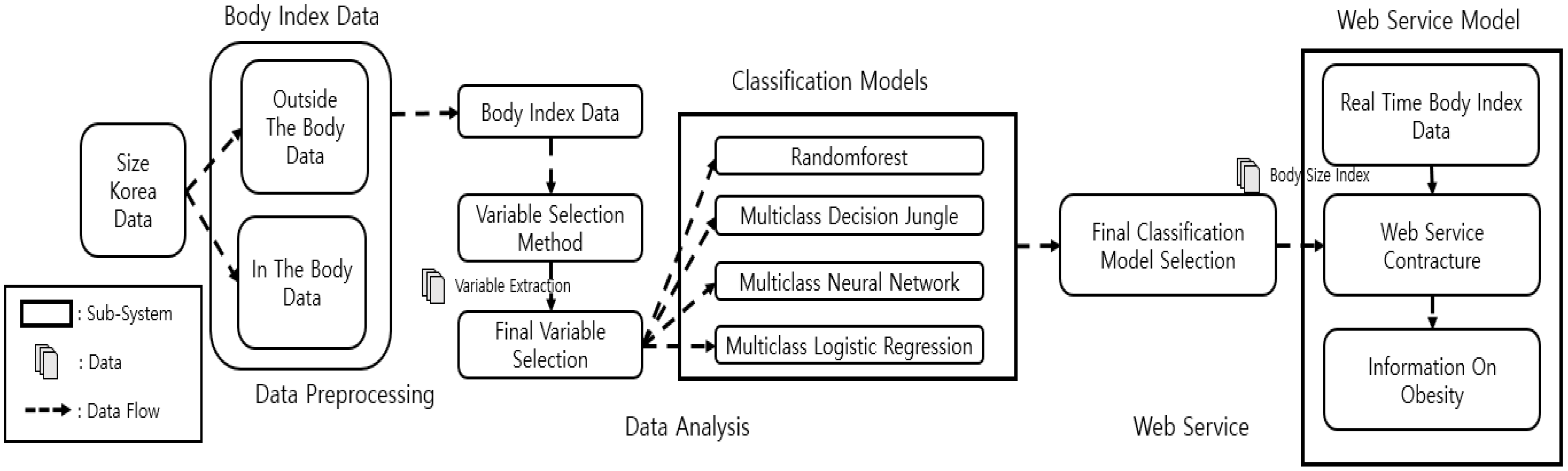
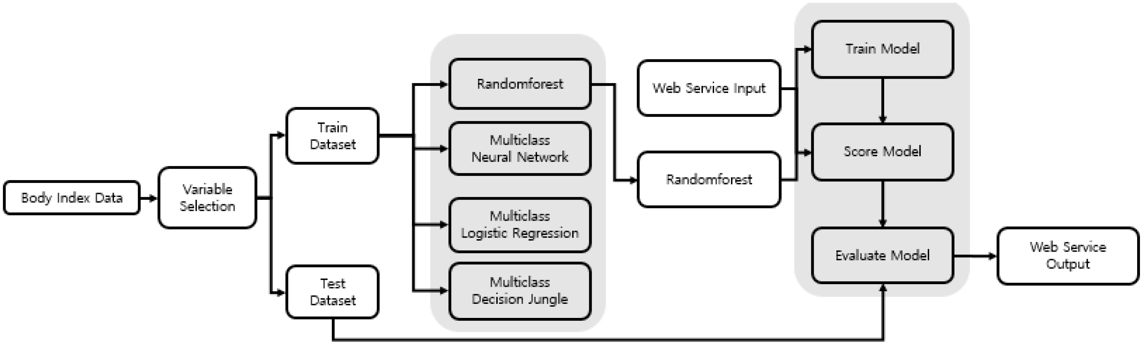
Figure 1 shows the overall process of this research, which comprises three stages: data preprocessing, data analysis, and web servicing. In the data preprocessing stage, the intracorporeal data were divided from the extracorporeal data (from Size Korea) into chest, waist, hip, arm, thigh, and calf, and the variables were selected using the variable selection model. We drew the final variables selected from the results of the variable selection. In the data analysis stage, we used the selected variables to create a total of four types of classification methods in order to find the model with the highest accuracy. After finding the model with the highest accuracy, in the web service stage, we built a web-based application that used body-part measurements and BMI information to show the obesity information. In the web services phase, information about obesity was derived from the models that were built in the data analysis phase and were configured based on the best model found.

3.3. Data Description and Feature Selection

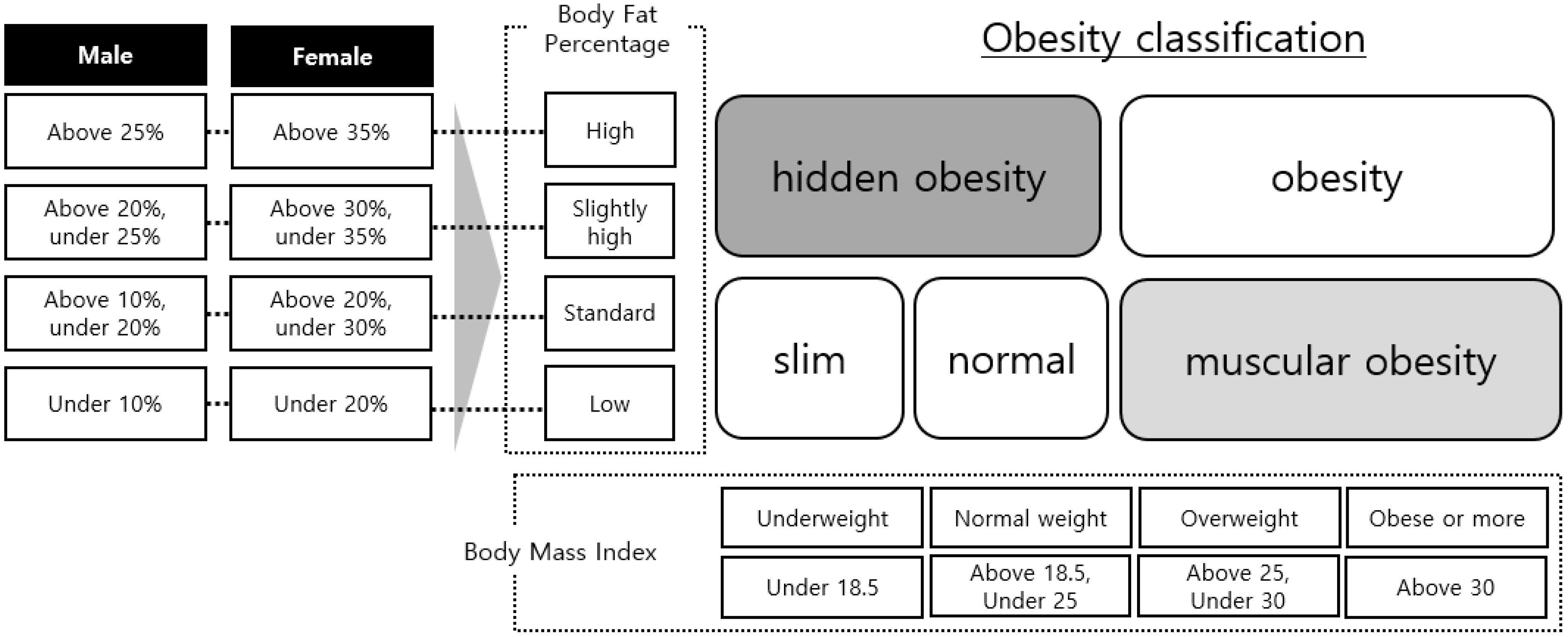
As shown in Figure 1, the information input identifies obesity based on the Size Korea data. The relationship between BMI and the BF percentage was identified, and a standard for obesity was established through WHO standards in that relationship [27]. As shown in Figure 2, we defined the BF ratio separately for men and women. Using the defined BF ratio information and BMI, we created five classes: slim, normal, hidden obesity, muscular obesity, and obesity. The drawn obesity information was converted to the following patterns: slim→underweight, normal→healthy range, hidden obesity→overweight, muscular obesity→obese, and obesity→obese, which were identical to the standard variables of BMI and WHtR, and were in line with the class values of BMI and WHtR to be compared.

We chose variables that affect obesity through a regression model, which is one of the ways in which we select variables. Since the regression model is the most widely used model to identify the relationships between the various numerical categorical independent variables for a single dependent variable, a variable selection was made using it. Therefore, a regression model was used to conduct variable selection, extracting variables from among 30 extracorporeal and intracorporeal variables that influence obesity. For the variable selection method, a stepwise regression, which is a multiple regression model, was used. In variable selection, we found the section with the highest adjusted $\mathrm{R}-\mathrm{Squared}$ value, and the section with the lowest $C_p$ value, to select the number of variables. Data preprocessing was completed by selecting the variables using the regression analysis.

The coefficient of determination in $\mathrm{R}-\mathrm{Squared}$ is an increasing function that also increases in size if the number of independent variables increases; thus, it has the disadvantage of the coefficient of determination increasing, regardless of significance, if the number of independent variables increases [28]. In adjusted $\mathrm{R}-\mathrm{Squared}$, the unexplained variation coefficient decreases and $n-p-1$ also decreases when the sum-of-square error increases, and is neither an increasing nor decreasing function, as shown in Equation (1); therefore, it is shown that adjusted $\mathrm{R}-\mathrm{Squared}$ is not an increasing function.

$$R_a^2=1-\frac{\left(n-1\right)\left(1-R^2\right)}{n-p-1}$$

(1)

The $C_p$ statistic value is a measure of how close the regression model of $p$ regressors is to the target model. We selected the model in which $C_p$ had the value closest to $p$ and had few variables in the p-regressor regression model [29].

$$C_p=\frac{SS{E}_p}{MSE}-n+2p$$

(2)

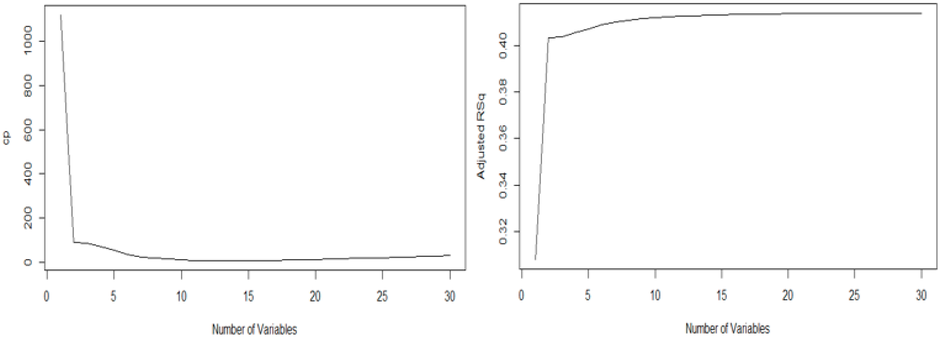
Therefore, the graphs of the $C_p$ statistic and the adjusted R-squared were each generated. Equation (2), which shows the sum of the residual squares (SSE) and the residual square mean (MSE), represents the sum of the residual squares of the model with each selected explanatory variable—the $p-\mathrm{value}$ is the number of explanatory variables selected and the $n$ value is the total number of explanatory variables. Therefore, this represents the estimator of the sum of the residual squares. Moreover, the minimum value of the $C_p$ statistic in this graph is 16, and the maximum value of the adjusted $\mathrm{R}-\mathrm{Squared}$ in this graph is also 16, as shown in Figure 3. Therefore, based on the above-mentioned two values, we performed optimal variable selection using the $p-\mathrm{value}$ in the regression analysis method. As a result, the following variables were selected for obesity analysis: gender, body-fat mass, body water, minerals, BMI, body-fat ratio, height, weight, waist circumference, hip breadth, hip vertical length, chest breadth, chest circumference, chest girth, thigh circumference, and calf circumference.

For the classification model, we used the following machine-learning methods to select the model with the highest accuracy as the final model: multiclass random forest, multiclass decision jungle, multiclass neural network, and multiclass logistic regression.

Table 4. Values of selected variables.

	Estimate	Std. Error	t Value	Pr (>|t|)
(Intercept)	0.1269347	0.8901940	0.143	0.886617
gender	1.0835835	0.0544733	19.892	<2 × 10−16
body-fat mass	−0.0135137	0.0075575	−1.788	0.073803
body water	−0.0253866	0.0081065	−3.132	0.001746
minerals	−0.0106529	0.0072712	−1.465	0.142945
BMI	0.1203787	0.0215231	5.593	2.32 × 10−8
body-fat ratio	−0.1133425	0.0045573	−24.870	2 × 10−16
height	0.0033897	0.0005686	5.961	2.64 × 10−9
weight	−0.0071550	0.0013629	−5.250	1.57 × 10−7
waist circumference	−0.0018812	0.0003692	−5.096	3.58 × 10−17
hip breadth	−0.0039953	0.0011944	−3.345	0.000828
Hip vertical length	−0.0014413	0.0006580	−2.190	0.028532
chest breadth	0.0016500	0.0010945	1.508	0.131721
chest circumference	−0.0011993	0.0004875	−2.460	0.013913
chest girth	0.0034860	0.0011075	3.148	0.001654
thigh circumference	−0.0009568	0.0006407	−1.493	0.135360
calf circumference	0.0012441	0.0008620	1.443	0.148994

shows that there are variables that have $p-\mathrm{values}$ that are not significant. However, because the optimal variable from the adjusted $\mathrm{R}-\mathrm{Squared}$ value and the $C_p$ statistic value were 16, we conducted the analysis using the variables drawn from variable selection.

3.4. Compare Methods

Random forest, one of the classification models, is an ensemble learning method. It outputs the classification, or mean predicted value, from the multiple decision trees that are built during the training process. One tree comprises a collection of nodes and edges in a hierarchical structure. Nodes are divided into internal nodes and terminal nodes. Therefore, it is a method to find the optimal model by using tree models that have different characteristics. When producing the first tree, the model measured the degree of inequality using the Gini coefficient in order to decide how many nodes were made. As the Gini coefficient approached 0, the distribution could be said to be equal; as it approached 1, the distribution was unequal. Therefore, in the case of the Gini coefficient decreasing, and the node’s impurity decreasing as the nodes separated, the division of the corresponding node was terminated, and the final tree model was made. Finally, the best model was drawn from the trees made in such a manner using the out-of-bag (OOB) method. When n observed samples are sampled with replacement n times, they are re-sampled with the probability of the following equation [30,31]. In Equation (3), by restoring n observation samples n times, the sample is capable of being duplicated in the sample, and the same size sample is taken as training data, with the other unselected objects being set as test sets. Therefore, the variables have slightly different characteristics for each tree and generalize the results, based on the predictions of each tree to improve performance. In this study, which deals with many variables, we used this method. In parameter setting of Random Forest trained each model through resampling method bagging and used 10 decision trees for training. In addition, the maximum depth of the tree was set to 32 and the number of random splits was set to 128, and 100 training was conducted.

$$\mathrm{OOB}=1-{(1-\frac{1}{n})}^n$$

(3)

Decision jungle is another ensemble model and is a method for detailed classification. This model refers to the combination of randomized ensembles of directed acyclic graphs (DAGs). This model has the function of a division node that obtains general information and the structure of DAGs. DAGs independently learn each root, and each root predicts accuracy using the learned nodes [32]. In parameter setting of multiclass decision jungle, ten decision directed acyclic graphs (DAGs) layers are used and the maximum depth of the decision tree was set to 32. Also, the number of optimization steps was defined as 2048.

Equation (4) applies to multiple class classification neural networks through Cross entropy. The value derived is the cost function E. The output $\mathrm{y}$ value ranges from $0<\mathrm{y}<1$ and the Cross entropy cost function is used together as an active function. $\mathrm{d}$ is displayed as one-hot-vector when the answer label is correct, and the error is equal to the output value to zero, and the larger the difference between the two values, the greater the error value. n and m mean the total number of $y_{ji}$ for each data, $\mathrm{i}-\mathrm{dimensional}$ value for the number of $\mathrm{j}$ data, and $d_{ji}$ means the $\mathrm{i}-\mathrm{dimensional}$ value. Thus, to calculate the probability for each data, the probability is expressed using ln, and the mean loss function is divided by $n$, which represents the total number of data. $\lambda$ is a cost function that determines how much the weight of the connection $\mathrm{w}$ will be reflected. Thus, even if the error is zero, the cost function will have a large value, thus solving the overcompatibility problem of the neural network by keeping the weight small.

$$\mathrm{E}=\frac{1}{N}{\displaystyle \sum }_j^n{\displaystyle \sum }_i^m\left\{-d_i\ln \left(y_{ji}\right)-\left(1-d_{ji}\right)\ln \left(1-y_{ji}\right)\right\}+\lambda \frac{1}{2}{\left|\left|w\right|\right|}^2$$

(4)

To minimize the costs after obtaining the cost function, the backpropagation algorithm was used. The accuracy of the classification model was obtained using the optimized cost function obtained through this process [33]. In parameter setting of multiclass neural network, there is no dropout where 100 hidden nodes are created, and all nodes are connected, and the learning rate is set to 0.001.

Logistic regression is a statistical methodology that is used to solve and predict the problem of identifying the linear relationship between independent and dependent variables, which is identical to the goal of a regular regression analysis. Logistic regression is used when the dependent variables are categorical data. When two or more dependent variables are analyzed, this is referred to as a multiclass logistic regression analysis. Logistic regression analysis faces the problem of effectively finding the linear predictor variables. Therefore, it can be represented as in Equation (5).

Logistic regression is a statistical method used to resolve and predict the problem of identifying linear relationships between independent and dependent variables just like the goals of regular regression. Logistic regression is used when the dependent variable is categorical data. Time to analyze more than one dependent variable is called multi-class logistic regression. Logistic regression is a good way to find linear predictors. Therefore, it can be expressed as in math Equation (5). The expression in logistic analysis is used to determine the effect of the regression values on the dependent variables by using a probability $p_x$ with anode ratio that indicates the intersection ratio and determines whether they are true or false, and thus the regression coefficients ${\beta }_0$, ${\beta }_n{x}_n$ and variables are used to determine the effect of the regression values of the various analysis variables on the dependent variables and to depend on the regression values that have the greatest influence on the data classification of data [34]. In parameter setting of multiclass logistic regression, four obesity information was designated as dependent variables, and through this, class prediction values for which data belong to each classification were derived. Multiclass logistic reserve derived 2.2 × 10⁻¹⁵ with $p-\mathrm{value}$ less than 0.05 and used it to select the model.

$${\log }_e\frac{p_x}{1-p_x}={\beta }_0+{\beta }_1{x}_1+{\beta }_2{x}_2+\cdots {\beta }_p{x}_{p.}$$

(5)

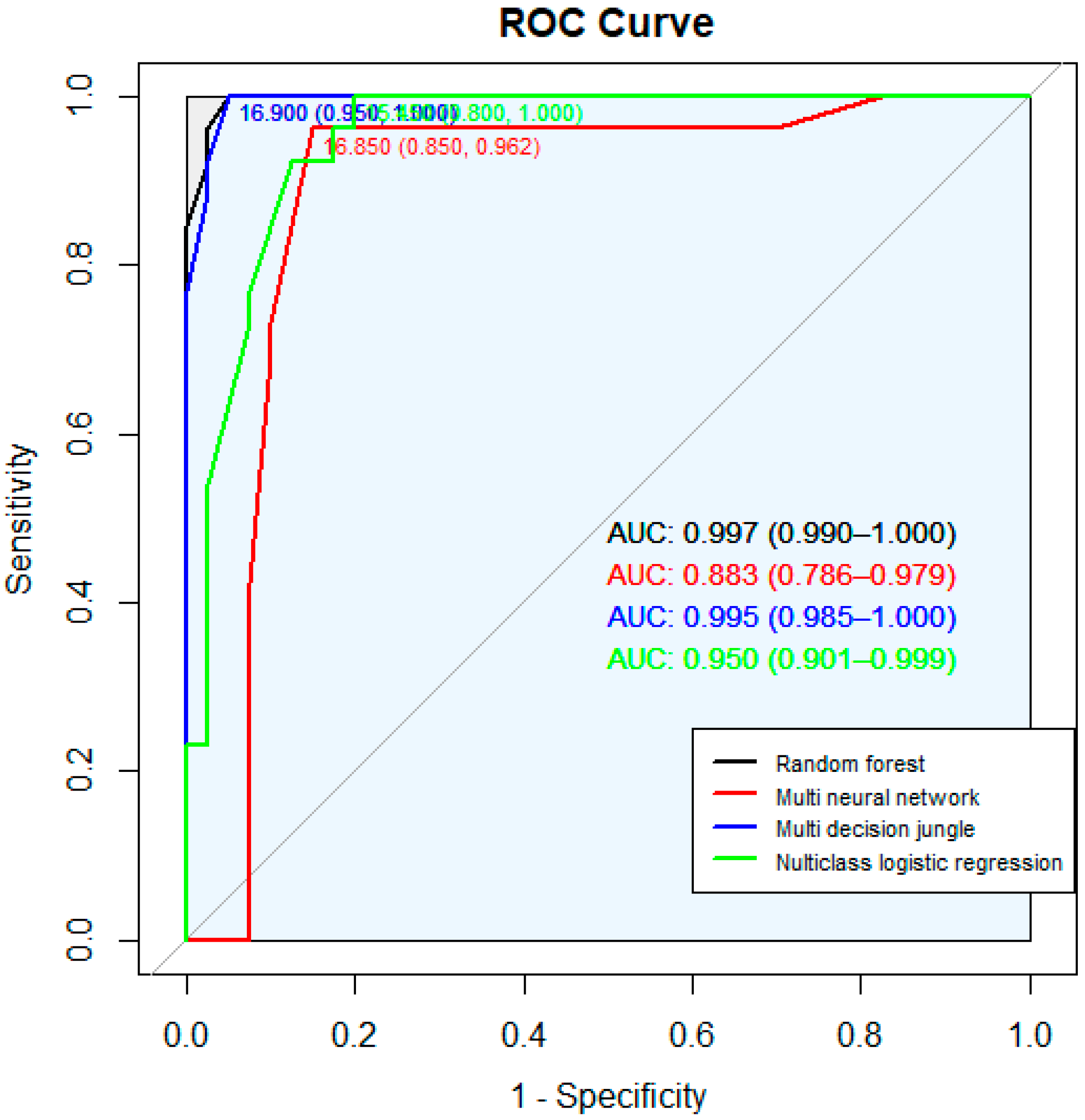
To select the model with the best value for deriving obesity information using these four models, the performance of the four models was judged using the accuracy of the model, the precision value, and the recall value.

Table 5. Results of classification analysis models.

Analysis Model	Accuracy	Precision	Recall
Random forest	0.99	0.99	0.99
Multiclass neural network	0.89	0.83	0.62
Multiclass decision jungle	0.99	0.99	0.99
Multiclass logistic regression	0.95	0.91	0.83

lists the accuracies of the four models. In Table 5, the accuracy of these data was derived by randomly extracting 100 data for four types of obesity information in order to select the model that produces the highest accuracy for the four classification models and the model that derives the highest accuracy for the obesity information. As a result, a total of 100 data were derived for the four obesity information (normal weight: 40, underweight: 26, overweight: 20, obese: 14) and random forest and multiclass decision jungle produced the highest accuracy and chose the random forest model. The values extracted from Table 5 are the representations of the average values of the four types of obesity information. Therefore, as shown in Figure 4, each ROC curve for each of the four models was derived, and the random forest with the highest accuracy was selected as the final model.

4. Results and Discussion

Using the selected variables and the four types of models, we generated each classification model, and then selected the most accurate model. In the analysis, we used the Azure statistics module provided by Microsoft, based on R. For the analysis models, we used the multiclass random forest, multiclass decision jungle, multiclass neural network, and multiclass logistic regression. Prior to analyzing each classification model, we conducted a model construction. Here, we modified the construction values so that all the models had identical conditions.

Random forest: This is a resampling method known as bagging, which is used to select multiple samples and trains them to each model in order to aggregate the result. We used ten decision trees; the maximum depth of the decision tree was set to 32; the number of random splits per node was set to 128; and the minimum number of samples per leaf node was defined as one. Bagging performs a restoration random sampling of the target data and sorts the extracted data into a sample group, which then collects the predictor variables of the learned models in order to generate a model [31] the multiclass neural network. For this, we set the hidden layer specification to be a fully connected case, with 100 hidden nodes being generated, and the learning rate was defined as 0.001. We performed 100 iterations. As with random forest, the resampling for the multiclass decision jungle model was completed via bagging. Ten decision DAGs were used. The maximum depth of the decision DAGs were set to 32, the number of random splits per node was set to 128, and the number of optimization steps per decision DAG layer was defined as 2048.

Multiclass logistic regression model: This was defined by using a value of 20 as the limited-memory Broyden Fletcher Goldfarb Shanno (L-BFGS) memory size. After defining the models, as mentioned, analyses were conducted. The analysis process was generated, as shown in Figure 5.

The total number of data values in the analysis models was 6382, which is divided into a Train set (70%) and a Test set (30%). A total of 16 variables were used to conduct the analyses. A total of 16 variables were used to conduct the analyses. 16 variables were used in the analysis using the variables shown in Table 4, and 16 variables included body-specific variables affecting obesity information and extracorporeal information affecting obesity. We aimed to select the model with the highest accuracy from among the four models in order to conduct obesity information extraction through body size information. Table 5 lists the accuracies of the four models. The values extracted from Table 5 are the representations of the average values of the four types of obesity information.

The results from evaluating the four levels of accuracy in the obesity information from each model showed that random forest produced the highest accuracy. Therefore, we used that model to machine-learn the data for the 16 variables (nine external variables: information including body length information and circumference information. Seven internal variables: information on the body’s internal body characteristics and numbers) and used this learning model to conduct obesity-information extraction using the extracorporeal data. Out of 16, 11 extracorporeal data variables were used, excluding intracorporeal data—fat mass, body water, minerals, BMI, and body fat (%)—in order to conduct a prediction analysis of obesity information. Based on real-time results, we used the Azure web application via the construction, in the process shown in Figure 5, to generate the web service process.

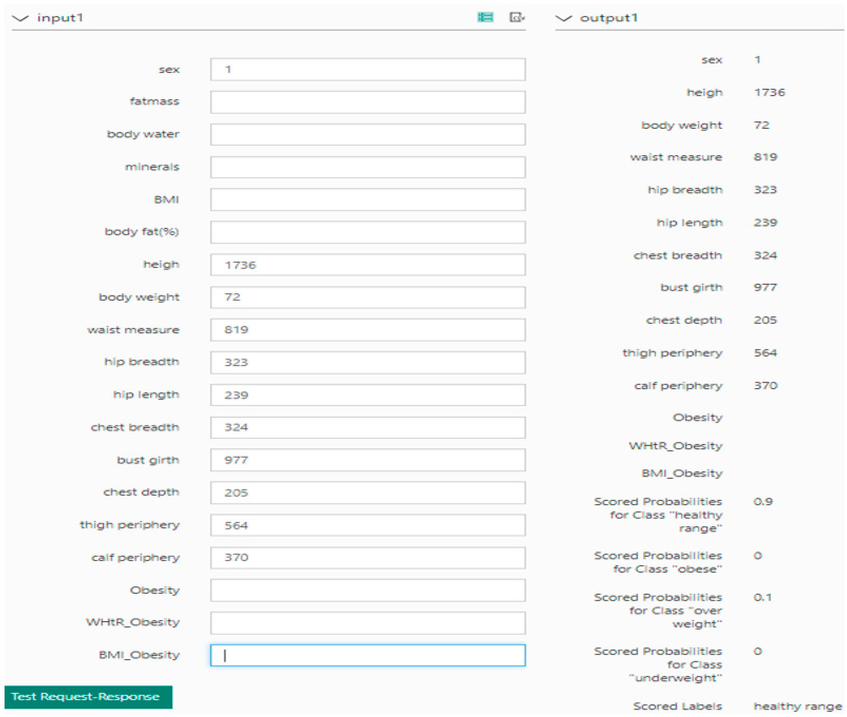
The prediction results using the process shown in Figure 5 in the Azure web environment are shown in Figure 6. In Figure 6, when the values are entered, the value of the Web Service input is then input to the value of the Score model, which is produced by the train model. The output value in the Web service is derived from the value received by the score model, in the Train model, as the output value in the Web service. Test data were randomly extracted 100 times from the data collected in 2014 from Size Korea, such as analysis data and the conducted tests.

The results using information learned from the random forest model and the body index data entered into the web page showed that obesity information was accurately predicted in 85 out of the 100 extracorporeal data values tested. Further, when we compared the histograms and boxplot with the obesity information, based solely on BMI and WHtR, the values from the obesity information differed greatly, and the comparison of the boxplot for each of the obesity measures, based on the BMI values, revealed different values and criteria. Depending on the measurement method, the obesity information extracted was shown to be different. The standards for BMI were defined as follows: (a) underweight: BMI < 18.5 kg/m²; (b) healthy range: 18.5 kg/m² ≤ BMI < 23.0 kg/m²; (c) overweight: 23.0 kg/m² ≤ BMI < 25.0 kg/m²; and (d) obese: 25.0 kg/m² ≤ BMI. The standards for WHtR were defined as follows: (a) underweight: WHtR < 0.43; (b) healthy range: 0.43 ≤ WHtR ≤ 0.53; (c) overweight: 0.53 ≤ overweight ≤ 0.58; and (d) obese, 0.58 ≤ obese.

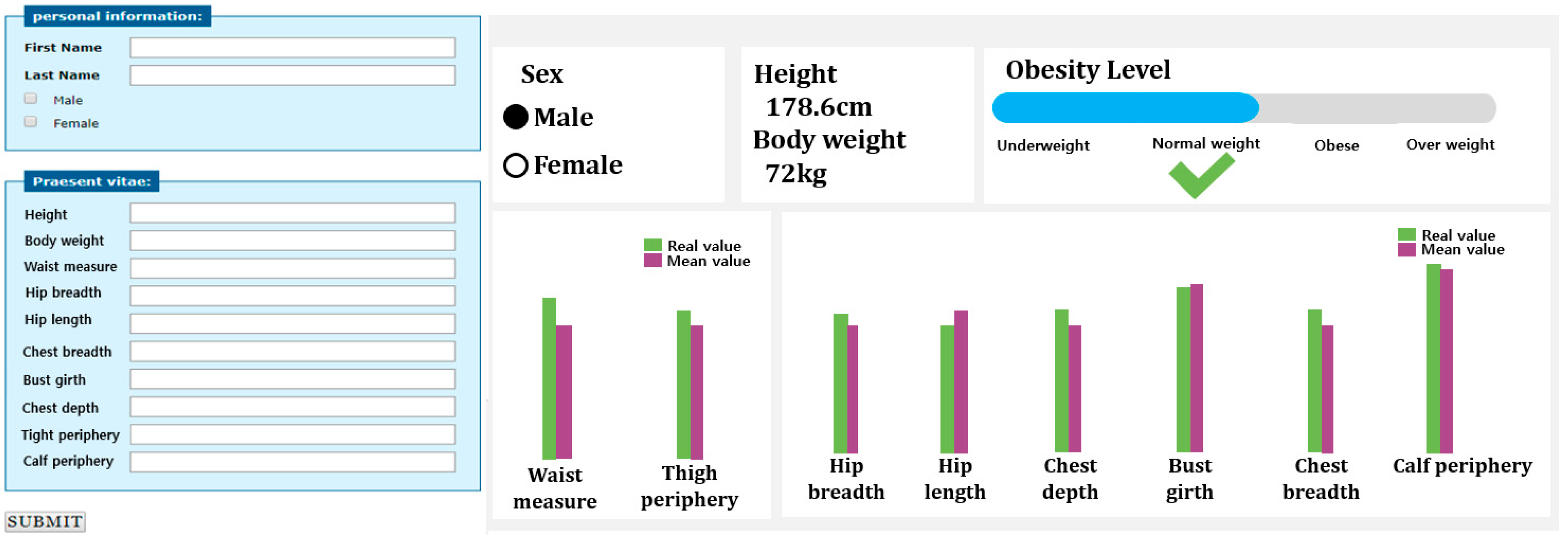
Figure 7 shows the webpage environment using the model created in Figure 6. Therefore, if you enter 10 body sizes and press submit, the obesity information is displayed using the model that has already been learned. Therefore, by using this webpage, you can understand your own obesity information in real time and update your information in real time.

5. Conclusions

As it is difficult to obtain precise information about obesity by only using values based on existing BMI and WHtR calculations, our study used machine learning from intracorporeal and extracorporeal information to more accurately measure obesity. For measurement data, we analyzed direct-measurement anthropomorphic data from the 2015 dataset of Size Korea. The structure of the data used in the analysis comprised of 148 variables for 6413 subjects (3192 men and 3221 women) in people aged from their 20s to 60s. For measurements in the investigation protocol for data collection, we considered the statistical method to decide measurement subjects based on ISO 15535, to calculate the minimum number of measurement subjects by relative accuracy (1–3%), using the maximum variation value of data by body type.

For the data, the body-data measuring tools used were rulers and body composition analyzers that can measure various body parts. The selection of variables was in two large groups: intracorporeal and extracorporeal data. For this study, we used the variables of skeletal muscle mass, body-fat mass, body water, minerals, body-fat ratio, and basal metabolism. For the analysis variables, we considered six parts of the human body: chest, waist, hip, arm, thigh, and calf. We then conducted the analysis using breadth, circumference, height, and girth of each part.

Prior to performing the analyses, we selected the variables using a regression model. Therefore, the graphs from the $C_p$ statistic and the adjusted R-squared were each generated. The minimum value of the $C_p$ statistic in this graph was 16, and the maximum value of the adjusted R-squared in this graph was also 16. Therefore, we selected 16 variables, from among 30, for the value that had the lowest value of the $C_p$ statistic and the highest value of the adjusted R-squared. The selected variables for the final analysis were gender, body-fat mass, body water, minerals, BMI, body-fat ratio, height, weight, waist circumference, hip breadth, hip vertical length, chest breadth, chest circumference, chest girth, thigh circumference, and calf circumference. We experimented with four analysis models: multiclass random forest, multiclass decision jungle, multiclass neural network, and multiclass logistic regression. Prior to analyzing each classification model, we conducted model construction. Here, we modified the construction values so that all the models had identical conditions.

As the final analysis model that proceeded to machine learning, we selected the random forest model because it had the highest accuracy from among the four models. After machine learning, we used the learned model and 11 variables, with only extracorporeal data, to predict obesity information. Further, we made a web-based application that could draw conclusions from the obesity information values entered by users. In this web calculator, predictions of the four levels of obesity, as shown in

Table 6. Obesity information comparison results.

	BMI	Body Fat (%)	WHR	WHtR	Web Application
Normal weight (Predicted value)	42% (70)	64% (75)	56% (62)	75% (82)	94% (97)
Underweight (Predicted value)	54% (132)	67% (121)	72% (123)	56% (103)	86% (95)
Overweigh (Predicted value)	46% (51)	78% (82)	64% (76)	62% (84)	92% (95)
Obese (Predicted value)	68% (147)	79% (122)	70% (139)	85% (131)	87% (113)

, and each of the 100 data values for web applications proposed in this paper, were predicted accurately, with an average of 90%. Table 6 extracts 100 of data for each of the four types of obesity information (normal weight, underweight, overweight, and obese) and compares them with the existing obesity measurement method and the web application presented in this study. In comparison, BMI, body fat percentage, WHR, WHtR, and Web applications proposed in this study were compared with four types of obesity, and accuracy was compared for a total of 400 data using 100 data each with four types of obesity information. Therefore, five methods of eliciting obesity information were compared for a total of 400 data, and the results are shown in Table 6. Therefore, we provided a predicted value of the accuracy of each measurement and how much information was classified for the measurement.

Using the final model, simple extracorporeal information, such as height, shoulder width, and weight, can be entered into the development system so that obesity can be derived, based on existing intracorporeal and extracorporeal information.

With the prediction of obesity information using extracorporeal information, real-time measurement of obesity can be made, and people can quickly receive and update their own obesity information without using high-cost equipment to measure physical information (e.g., an Inbody machine or body-composition analyzer). Our web-based obesity calculator is convenient for self-diagnosis, incurs almost no cost, and is not restricted by a user’s location. Therefore, unlike previous measurement methods, which are great for height, weight, and one characteristic of the body, this method incorporates information from various body parts and provides an obesity decision that is based on the model learned from this information. By creating a model using intracorporeal and extracorporeal data, a higher accuracy of obesity can be derived than when only using extracorporeal data. Therefore, it was possible to predict obesity more accurately than the existing method, which only assesses obesity through one value, such as height, weight, and waist circumference. With the new method, it was possible to find that body composition is normal, even though it had been shown to be hidden and muscular. However, this study focuses on Korean data to diagnose obesity according to Korean characteristics. Therefore, the failure to analyze various countries is a limitation of this study, and a better study in the future would design and analyze the criteria for obesity information in various countries. In addition, as more information about obesity and related data is collected, we expect that further research will be conducted.