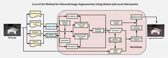
A Level Set Method for Infrared Image Segmentation Using Global and Local Information

 ,
, 


Abstract
:
1. Introduction
- a new SPF integrating both global-intensity-based information and local-multi-feature-based information via an adaptive weight matrix is developed;
- four statistical features are dynamically weighted by range ratio to form the driving force which is utilized to form the local term of SPF;
- a level set formula which is able to cope with the weak edge and intensity inhomogeneity is constructed using the SPF proposed;
- the segmentation results are not obviously influenced by the initialization of contour.
2. Related Work about Geodesic Active Contour (GAC) Model
3. Theory
3.1. Signed Pressure Fucntion Integrating Global and Local Information
3.1.1. Design of the Global Term
3.1.2. Design of the Local Term
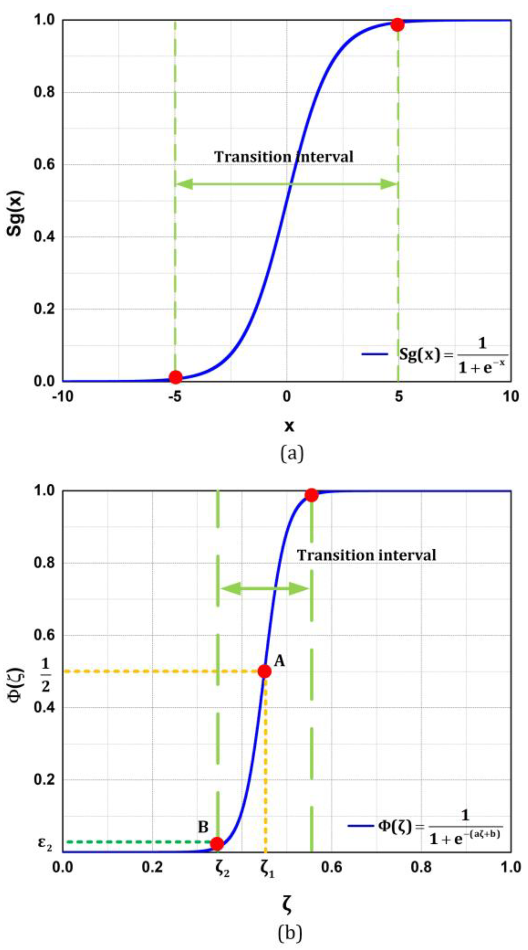
3.1.3. Combination of Global and Local Terms
- it should be a non-negative and monotonically increasing function;
- and , where and denote the maximum and minimum in the range matrix .
3.2. Implementation
3.2.1. Initialization of Level Set Function
3.2.2. Construction of Level Set Formula
3.2.3. Evolution of Level Set Function
3.3. Summary of the Proposed Method
| Algorithm 1 Level set method using global and local information |
| Input: an IR image |
| 1. Initialization: initialize the level set function to be a binary function using Equation (28). |
| 2. While not convergence do |
| 3. for each pixel do |
| 4. Calculate the global term of SPF using Equation (6) |
| 5. Calculate the local term of SPF using Equation (23) |
| 6. Calculate the adaptive weight matrix using Equation (25) |
| 7. Combing and to construct SPF using Equation (24) |
| 8. end 9. Construct the level set formulation according to Equation (30) |
| 10. Evolve according to Equation (31) |
| 11. Let , if ; otherwise, |
| 12. Regularize using a Gaussian kernel function according to Equation (32) |
| 13. if |
| 14. break |
| 15. end if |
| 16. end |
| Output: The resulting contour . |
4. Experiment and Discussion
4.1. Parameter Setting
4.1.1. Parameter Description
4.1.2. Sensitivity Analysis
4.2. Comparative Experiment
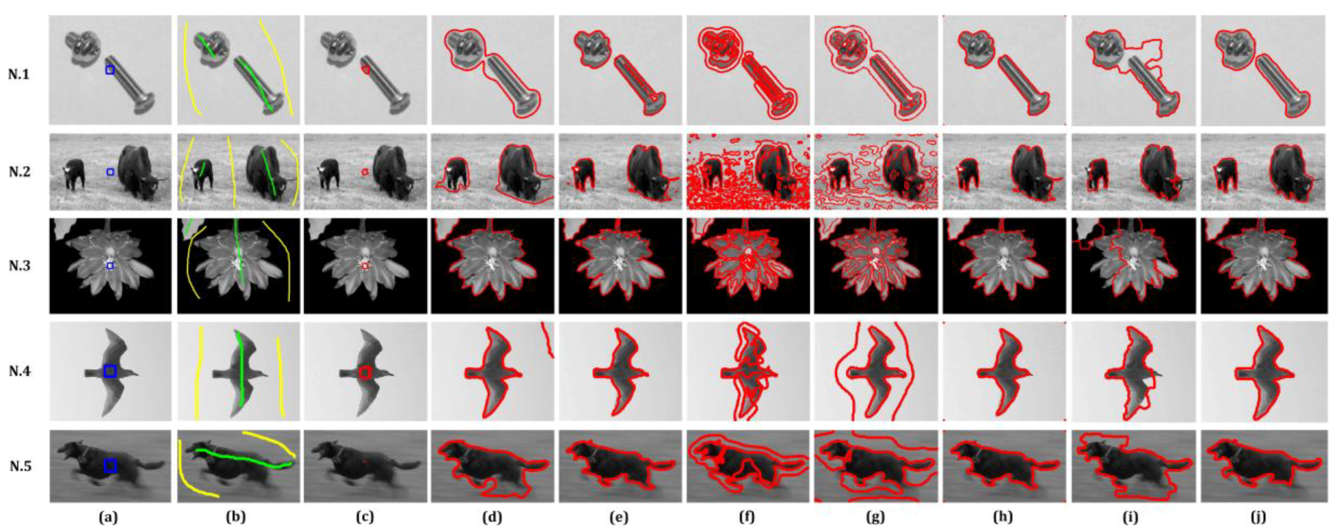
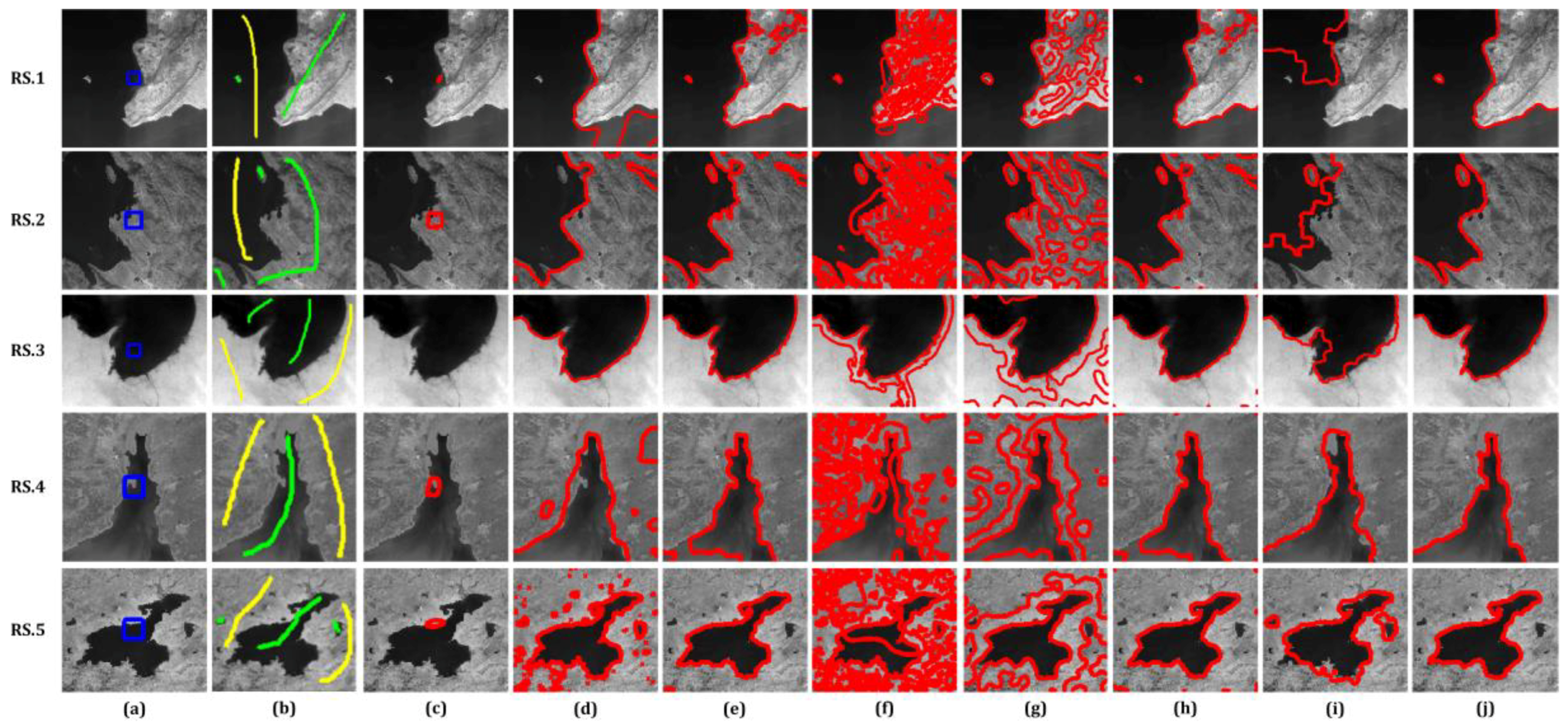
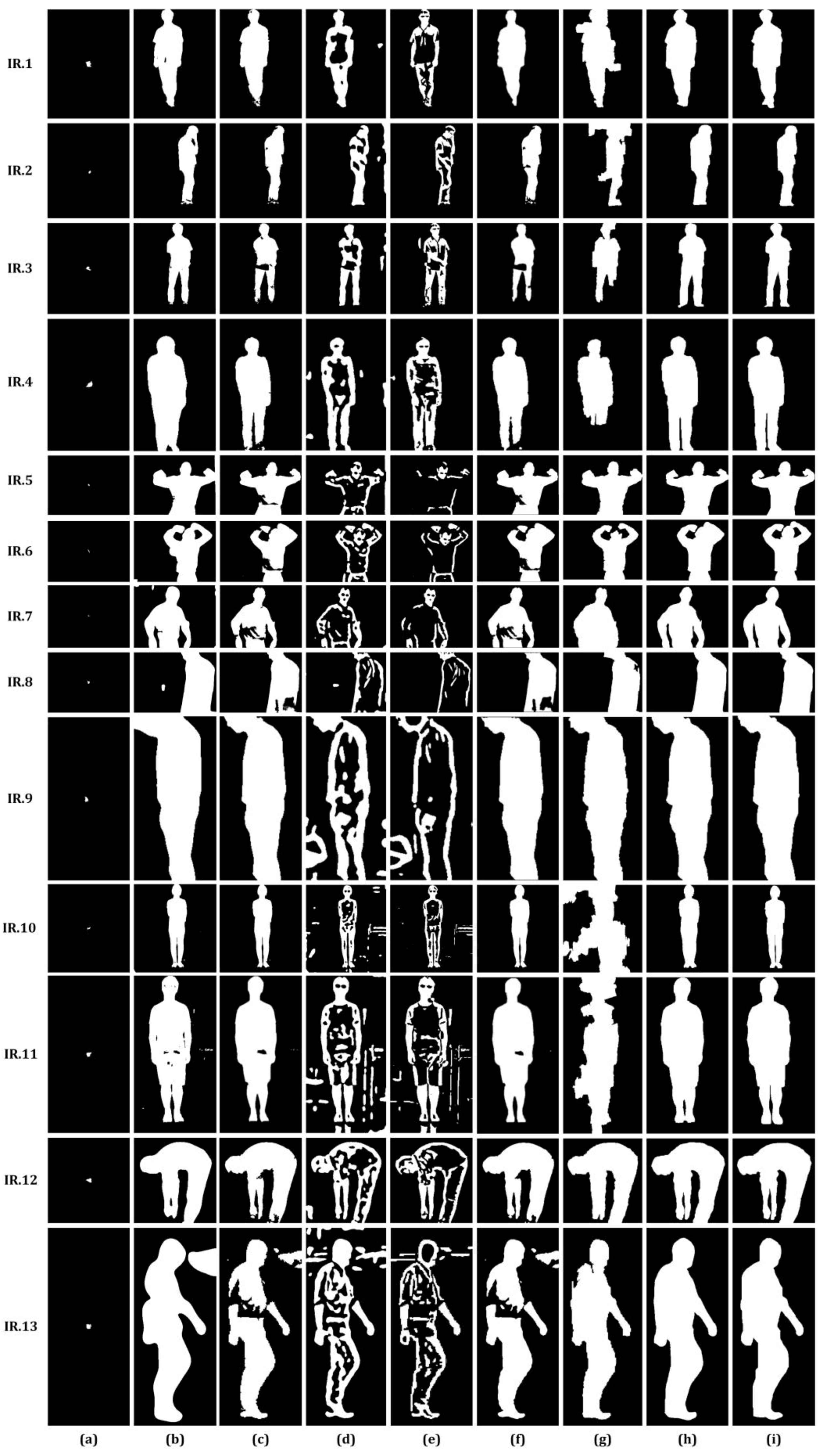
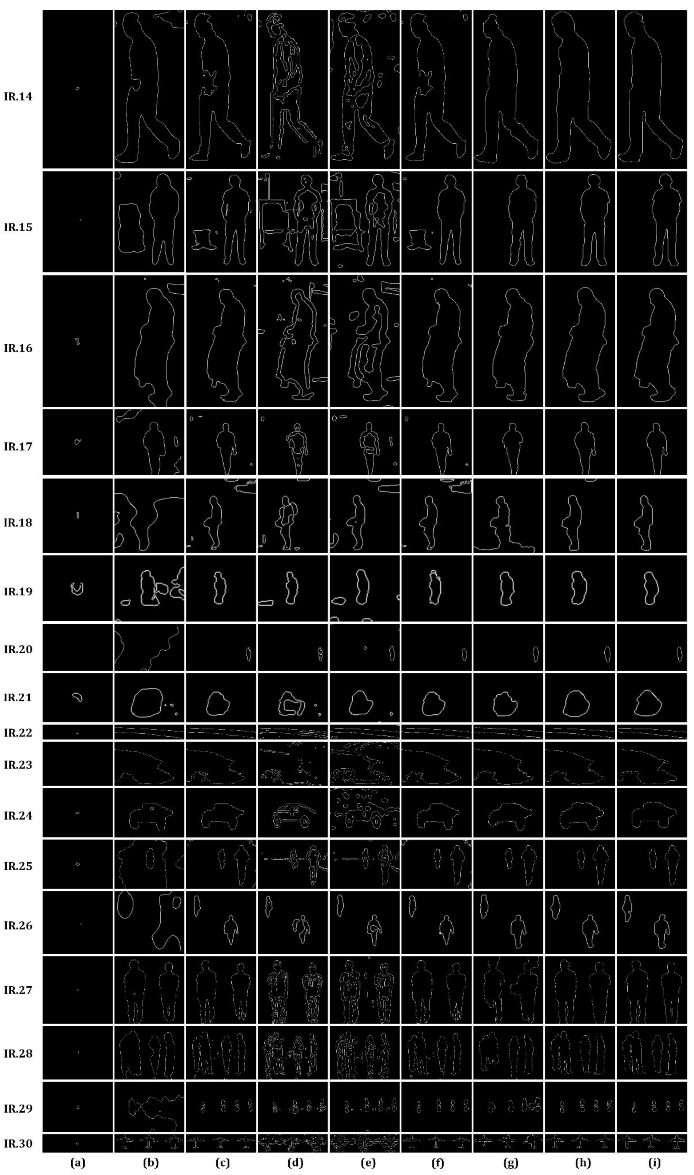
4.2.1. Segmentation Result
4.2.2. Comparison of Segmentation Accuracy
4.2.3. Comparison of Running Time
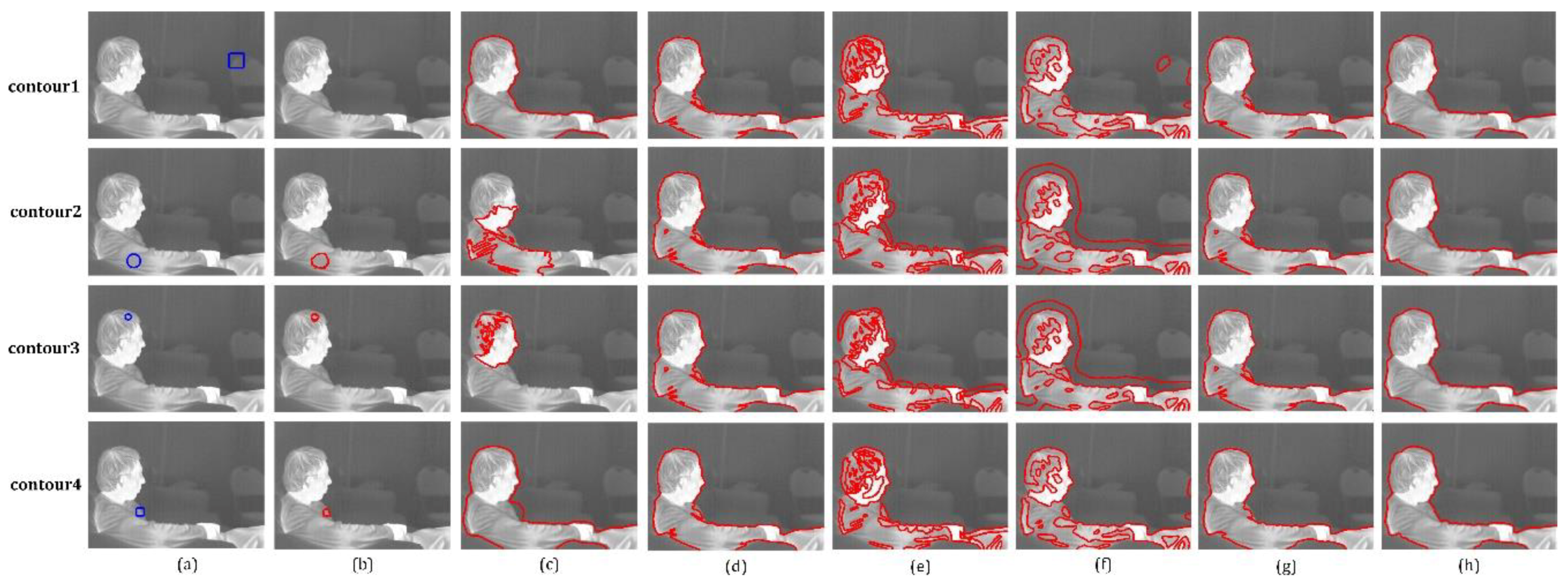
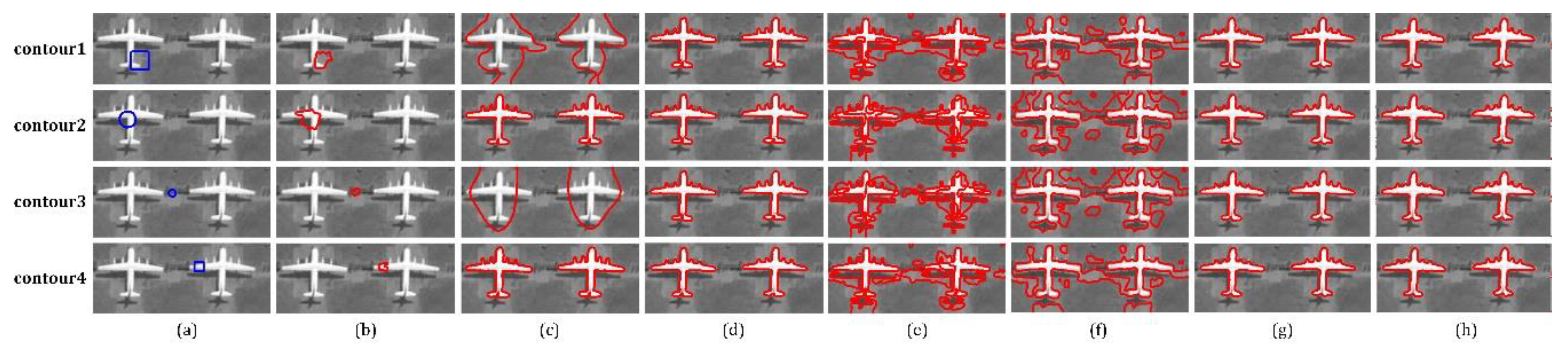
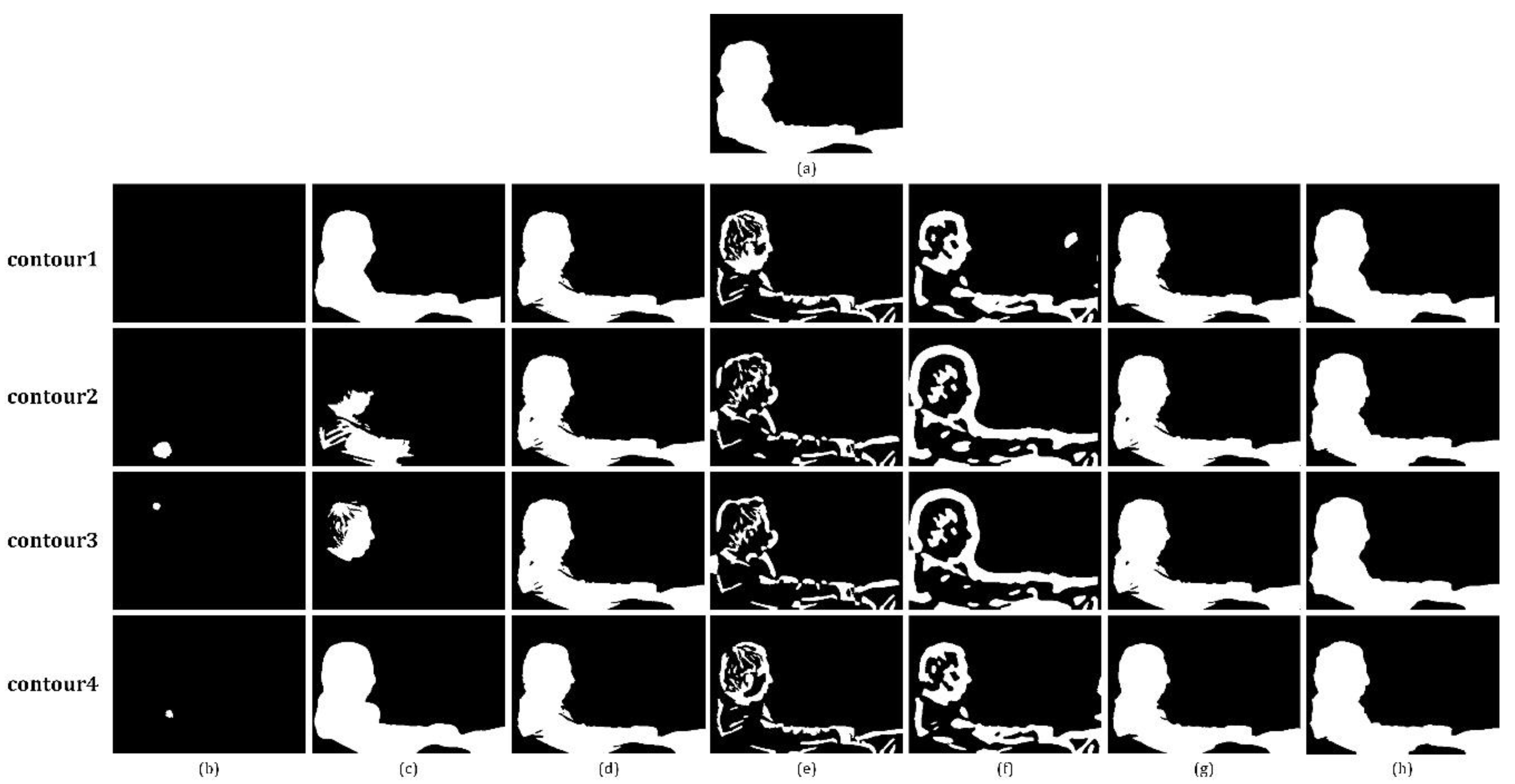
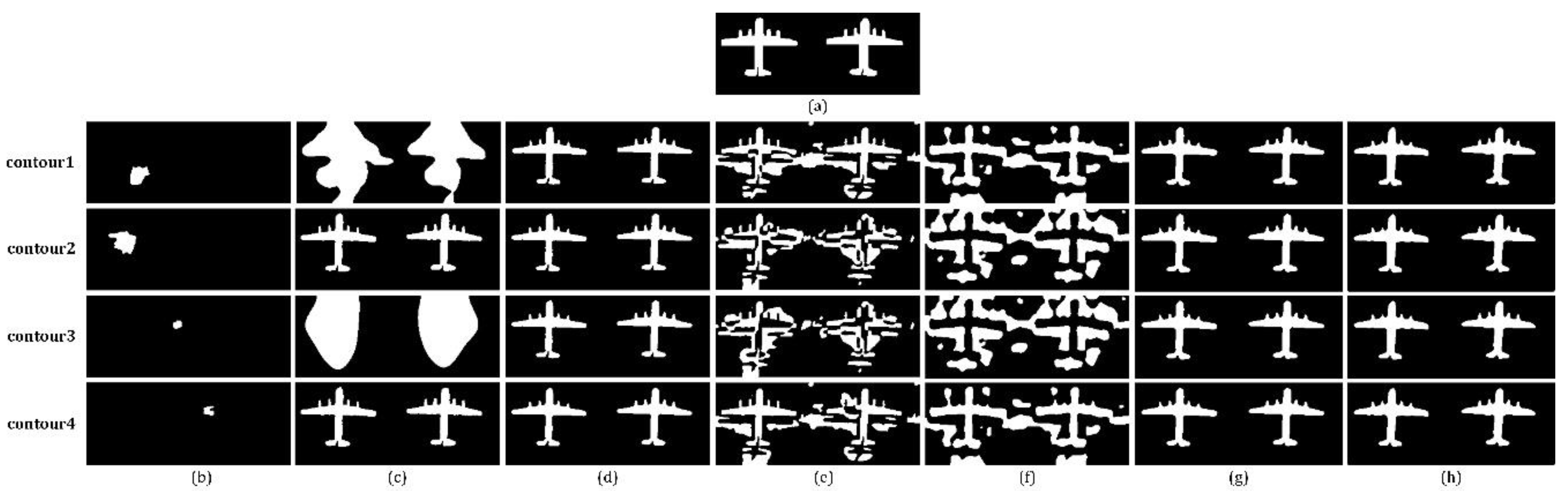
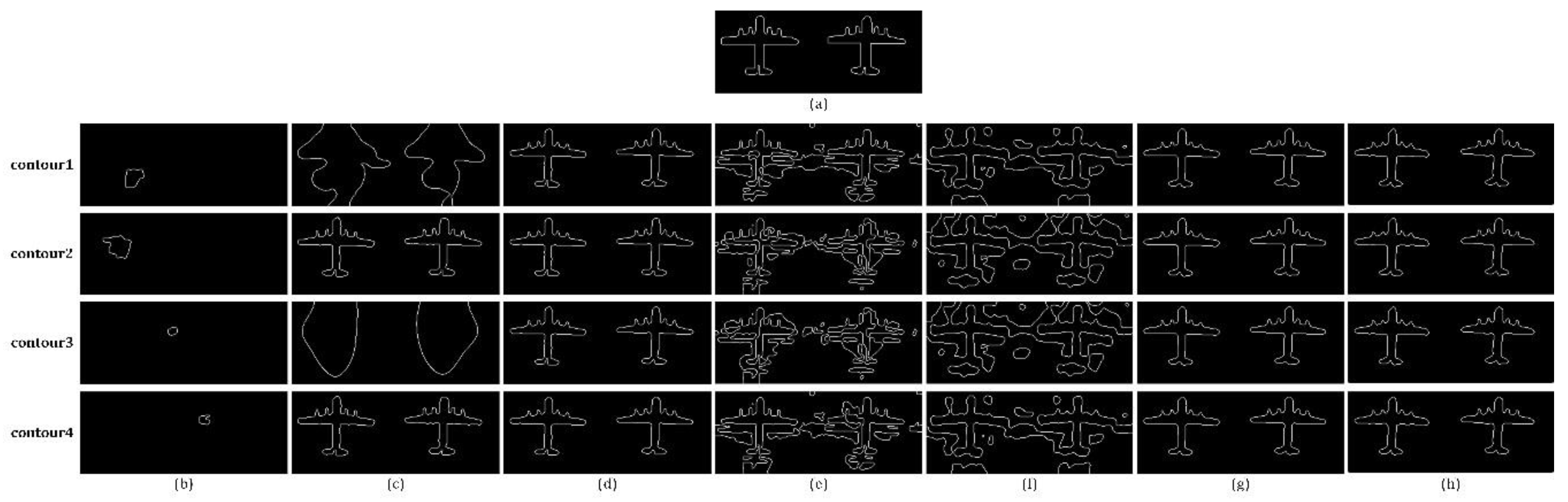
4.2.4. Influence of Contour Initialization
5. Conclusions
5.1. Methdology
5.2. Applicability and Limitation to Remote Sensing
5.3. Future Work
Author Contributions
Funding
Conflicts of Interest
References
- Huang, J.; Ma, Y.; Zhang, Y.; Fan, F. Infrared image enhancement algorithm based on adaptive histogram segmentation. Appl. Opt. 2017, 56, 9686–9697. [Google Scholar] [CrossRef] [PubMed]
- Zingoni, A.; Diani, M.; Corsini, G. A Flexible Algorithm for Detecting Challenging Moving Objects in Real-Time within IR Video Sequences. Remote Sens. 2017, 9, 1128. [Google Scholar] [CrossRef]
- Lei, S.; Zou, Z.; Liu, D.; Xia, Z.; Shi, Z. Sea-land segmentation for infrared remote sensing images based on superpixels and multi-scale features. Infrared Phys. Technol. 2018, 91, 12–17. [Google Scholar] [CrossRef]
- Wan, M.; Gu, G.; Qian, W.; Ren, K.; Chen, Q.; Maldague, X. Particle swarm optimization-based local entropy weighted histogram equalization for infrared image enhancement. Infrared Phys. Technol. 2018, 91, 164–181. [Google Scholar] [CrossRef]
- Pal, N.R.; Pal, S.K. A review on image segmentation techniques. Pattern Recognit. 1993, 26, 1277–1294. [Google Scholar] [CrossRef]
- Lee, L.K.; Liew, S.C.; Thong, W.J. A review of image segmentation methodologies in medical image. In Advanced Computer and Communication Engineering Technology; Springer: New York, NY, USA, 2015; pp. 1069–1080. [Google Scholar]
- Niu, S.; Chen, Q.; de Sisternes, L.; Ji, Z.; Zhou, Z.; Rubin, D.L. Robust noise region-based active contour model via local similarity factor for image segmentation. Pattern Recognit. 2017, 61, 104–119. [Google Scholar] [CrossRef]
- Cao, J.; Wu, X. A novel level set method for image segmentation by combining local and global information. J. Mod. Opt. 2017, 64, 2399–2412. [Google Scholar] [CrossRef]
- Caselles, V.; Kimmel, R.; Sapiro, G. Geodesic active contours. Int. J. Comput. Vis. 1997, 22, 61–79. [Google Scholar] [CrossRef]
- Tian, Y.; Duan, F.; Zhou, M.; Wu, Z. Active contour model combining region and edge information. Mach. Vis. Appl. 2013, 24, 47–61. [Google Scholar] [CrossRef]
- Melonakos, J.; Pichon, E.; Angenent, S.; Tannenbaum, A. Finsler active contours. IEEE Trans. Pattern Anal. Mach. Intell. 2008, 30, 412–423. [Google Scholar] [CrossRef] [PubMed]
- Paragios, N. Variational methods and partial differential equations in cardiac image analysis. In Proceedings of the IEEE International Symposium on Biomedical Imaging: Nano to Macro, Arlington, VA, USA, 15–18 April 2004; pp. 17–20. [Google Scholar]
- Wang, D.; Zhang, T.; Yan, L. Fast hybrid fitting energy-based active contour model for target detection. Chin. Opt. Lett. 2011, 9, 071001-071001. [Google Scholar] [CrossRef]
- Zhao, W.; Xianze, X.; Zhu, Y.; Xu, F. Active contour model based on local and global Gaussian fitting energy for medical image segmentation. Opt. Int. J. Light Electron. Opt. 2018, 158, 1160–1169. [Google Scholar] [CrossRef]
- Chan, T.F.; Vese, L.A. Active contours without edges. IEEE Trans. Image Process. 2011, 10, 266–277. [Google Scholar] [CrossRef] [PubMed]
- Mumford, D.; Shah, J. Optimal approximations by piecewise smooth functions and associated variational problems. Commun. Pure Appl. Math. 1989, 42, 577–685. [Google Scholar] [CrossRef] [Green Version]
- Wang, Y.; Huang, T.Z.; Wang, H. Region-based active contours with cosine fitting energy for image segmentation. J. Opt. Soc. Am. A Opt. Image Sci. Vis. 2015, 32, 2237–2246. [Google Scholar] [CrossRef] [PubMed]
- Tsai, A.; Yezzi, A.; Willsky, A.S. Curve evolution implementation of the Mumford-Shah functional for image segmentation, denoising, interpolation, and magnification. IEEE Trans. Image Process. 2001, 10, 1169–1186. [Google Scholar] [CrossRef] [PubMed]
- Vese, L.A.; Chan, T.F. A multiphase level set framework for image segmentation using the Mumford and Shah model. Int. J. Comput. Vis. 2002, 50, 271–293. [Google Scholar] [CrossRef]
- Zhang, K.; Zhang, L.; Song, H.; Zhou, W. Active contours with selective local or global segmentation: A new formulation and level set method. Image Vis. Comput. 2010, 28, 668–676. [Google Scholar] [CrossRef]
- Li, C.; Kao, C.Y.; Gore, J.C.; Ding, Z. Minimization of region-scalable fitting energy for image segmentation. IEEE Trans. Image Process. 2008, 17, 1940–1949. [Google Scholar] [PubMed]
- Zhang, K.; Xu, S.; Zhou, W.; Liu, B. Active contours based on image Laplacian fitting energy. Chin. J. Electron. 2009, 18, 281–284. [Google Scholar]
- Wang, L.; Pan, C. Robust level set image segmentation via a local correntropy-based K-means clustering. Pattern Recognit. 2014, 47, 1917–1925. [Google Scholar] [CrossRef]
- Wang, L.; Li, C.; Sun, Q.; Xia, D.; Kao, C.Y. Active contours driven by local and global intensity fitting energy with application to brain MR image segmentation. Comput. Med. Imaging Graph. 2009, 33, 520–531. [Google Scholar] [CrossRef] [PubMed]
- Dong, F.; Chen, Z.; Wang, J. A new level set method for inhomogeneous image segmentation. Image Vis. Comput. 2013, 31, 809–822. [Google Scholar] [CrossRef]
- Zhao, Y.; Nie, X.; Duan, Y.; Huang, Y.; Luo, S. A benchmark for interactive image segmentation algorithms. In Proceedings of the IEEE Workshop on Person-Oriented Vision (POV), Kona, HI, USA, 7 January 2010; pp. 33–38. [Google Scholar]
- Panagiotakis, C.; Papadakis, H.; Grinias, E.; Komodakis, N.; Fragopoulou, P.; Tziritas, G. Interactive image segmentation based on synthetic graph coordinates. Pattern Recognit. 2013, 46, 2940–2952. [Google Scholar] [CrossRef]
- Ning, J.; Zhang, L.; Zhang, D.; Wu, C. Interactive image segmentation by maximal similarity based region merging. Pattern Recognit. 2010, 43, 445–456. [Google Scholar] [CrossRef]
- Veksler, O. Star shape prior for graph-cut image segmentation. In Proceedings of the European Conference on Computer Vision, Marseille, France, 12–18 October 2008; pp. 454–467. [Google Scholar]
- Gulshan, V.; Rother, C.; Criminisi, A.; Blake, A.; Zisserman, A. Geodesic star convexity for interactive image segmentation. In Proceedings of the IEEE Conference on Computer Vision and Pattern Recognition (CVPR), San Francisco, CA, USA, 13–18 June 2010; pp. 3129–3136. [Google Scholar]
- Zhi, X.H.; Shen, H.B. Saliency driven region-edge-based top down level set evolution reveals the asynchronous focus in image segmentation. Pattern Recognit. 2018, 80, 241–255. [Google Scholar] [CrossRef]
- Xu, C.; Yezzi, A.; Prince, J.L. On the relationship between parametric and geometric active contours. In Proceedings of the IEEE Conference Record of the Thirty-Fourth Asilomar Conference on Signals, Systems and Computers, Pacific Grove, CA, USA, 29 October–1 November 2000; pp. 483–489. [Google Scholar]
- Yu, Y.; Zhang, C.; Wei, Y.; Li, X. Active contour method combining local fitting energy and global fitting energy dynamically. In Proceedings of the International Conference on Medical Biometrics, Hong Kong, China, 28–30 June 2010; pp. 163–172. [Google Scholar]
- Wan, M.; Gu, G.; Qian, W.; Ren, K.; Chen, Q. Hybrid active contour model based on edge gradients and regional multi-features for infrared image segmentation. Opt. Int. J. Light Electron. Opt. 2017, 140, 833–842. [Google Scholar] [CrossRef]
- Zhang, T.; Han, J.; Zhang, Y.; Bai, L. An adaptive multi-feature segmentation model for infrared image. Opt. Rev. 2016, 23, 220–230. [Google Scholar] [CrossRef]
- Wan, M.; Gu, G.; Qian, W.; Ren, K.; Chen, Q. Infrared small target enhancement: Grey level mapping based on improved sigmoid transformation and saliency histogram. J. Mod. Opt. 2018, 65, 1161–1179. [Google Scholar] [CrossRef]
- Perona, P.; Malik, J. Scale-space and edge detection using anisotropic diffusion. IEEE Trans. Pattern Anal. Mach. Intell. 1990, 12, 629–639. [Google Scholar] [CrossRef] [Green Version]
- Wan, M.; Gu, G.; Qian, W.; Ren, K.; Chen, Q.; Maldague, X. Infrared Image Enhancement Using Adaptive Histogram Partition and Brightness Correction. Remote Sens. 2018, 10. [Google Scholar] [CrossRef]
- Mangale, S.A.; Khambete, M.B. Approach for moving object detection using visible spectrum and thermal infrared imaging. J. Electron. Imaging 2018, 27. [Google Scholar] [CrossRef]
- Peng, H.; Li, B.; Ling, H.; Hu, W.; Xiong, W.; Maybank, S.J. Salient object detection via structured matrix decomposition. IEEE Trans. Pattern Anal. Mach. Intell. 2017, 39, 818–832. [Google Scholar] [CrossRef] [PubMed]
- Database Collection of Infrared Image. Available online: http://www.dgp.toronto.edu/nmorris/IR/ (accessed on 16 June 2018).
- MSRA10K Salient Object Database. Available online: http://mmcheng.net/msra10k/ (accessed on 19 June 2018).
- Gu, Y.; Ren, K.; Wang, P.; Gu, G. Polynomial fitting-based shape matching algorithm for multi-sensors remote sensing images. Infrared Phys. Technol. 2016, 76, 386–392. [Google Scholar] [CrossRef]
- Gao, W.; Zhang, X.; Yang, L.; Liu, H. An improved Sobel edge detection. In Proceedings of the 2010 3rd IEEE International Conference on Computer Science and Information Technology (ICCSIT), Chengdu, China, 9–11 July 2010; pp. 67–71. [Google Scholar]


| Parameter | Meaning | Default Value |
|---|---|---|
| The control factor of Heaviside function | 1.5 | |
| m | The length of local window | 5 |
| The standard deviation of the Gaussian filter used for embedding local features | 3.0 | |
| Help to determine the magnitude of driving force | 1.5 | |
| Help to determine the central point of | 0.3 | |
| The value of the lower inflection point of | 0.00001 | |
| The balloon force of level set formula | 400 | |
| The constant utilized for initializing the contour | 1 | |
| The side length of initial contour | 7 | |
| The standard deviation of the Gaussian filter used for regularizing level set function | 2.5 | |
| The convergence threshold | 0.03 |
| GAC | CV | SBGFRLS | LBF | ILFE | Cao’s Model | MSRM | Ours | |
|---|---|---|---|---|---|---|---|---|
| IR. 1 | 0 | 0.9758 | 0.9378 | 0.3651 | 0.5069 | 0.9378 | 0.8742 | 0.9859 |
| IR. 2 | 0.0235 | 0.9359 | 0.9499 | 0.6582 | 0.8105 | 0.9624 | 0.7879 | 0.9664 |
| IR. 3 | 0.0143 | 0.9361 | 0.8886 | 0.7826 | 0.8101 | 0.8883 | 0.8538 | 0.9595 |
| IR. 4 | 0.0150 | 0.9310 | 0.9525 | 0.7479 | 0.7475 | 0.9517 | 0.8616 | 0.9837 |
| IR. 5 | 0.0029 | 0.9643 | 0.9376 | 0.2745 | 0.5536 | 0.9420 | 0.9794 | 0.9778 |
| IR. 6 | 0.0027 | 0.9522 | 0.9054 | 0.4377 | 0.6520 | 0.9020 | 0.9667 | 0.9683 |
| IR. 7 | 0.0013 | 0.9537 | 0.9157 | 0.4307 | 0.5986 | 0.9145 | 0.9406 | 0.9796 |
| IR. 8 | 0 | 0.9530 | 0.9311 | 0.7299 | 0.8118 | 0.9240 | 0.9729 | 0.9617 |
| IR. 9 | 0.0040 | 0.9351 | 0.9787 | 0.4946 | 0.7172 | 0.9745 | 0.9838 | 0.9876 |
| IR. 10 | 0.0073 | 0.9441 | 0.9445 | 0.6571 | 0.6941 | 0.9430 | 0.5016 | 0.9545 |
| IR. 11 | 0.0074 | 0.9643 | 0.9641 | 0.6066 | 0.6494 | 0.9662 | 0.8357 | 0.9783 |
| IR. 12 | 0.0093 | 0.9548 | 0.9458 | 0.6459 | 0.7411 | 0.9455 | 0.9740 | 0.9759 |
| IR. 13 | 0.0067 | 0.8941 | 0.8725 | 0.5946 | 0.7264 | 0.8717 | 0.9632 | 0.9695 |
| IR. 14 | 0.0031 | 0.9079 | 0.8843 | 0.5122 | 0.7632 | 0.8850 | 0.9525 | 0.9647 |
| IR. 15 | 0 | 0.7126 | 0.8598 | 0.5819 | 0.6197 | 0.8611 | 0.9660 | 0.9790 |
| IR. 16 | 0.0070 | 0.9271 | 0.9462 | 0.4711 | 0.7425 | 0.9468 | 0.9621 | 0.9679 |
| IR. 17 | 0.0556 | 0.7498 | 0.9306 | 0.6856 | 0.7073 | 0.9355 | 0.9415 | 0.9731 |
| IR. 18 | 0.0233 | 0.3638 | 0.7732 | 0.6572 | 0.7526 | 0.7861 | 0.6857 | 0.9296 |
| IR. 19 | 0.3222 | 0.5399 | 0.8920 | 0.7951 | 0.7114 | 0.8820 | 0.9191 | 0.9179 |
| IR. 20 | 0 | 0.0910 | 0.8594 | 0.7692 | 0.7802 | 0.8466 | 0.9041 | 0.9128 |
| IR. 21 | 0.1585 | 0.7905 | 0.8954 | 0.6074 | 0.8835 | 0.8954 | 0.9123 | 0.9637 |
| IR. 22 | 0.0018 | 0.9564 | 0.9677 | 0.8712 | 0.9307 | 0.9677 | 0.9542 | 0.9642 |
| IR. 23 | 0 | 0.9543 | 0.9597 | 0.1782 | 0.4665 | 0.9606 | 0.9662 | 0.9640 |
| IR. 24 | 0.0100 | 0.9007 | 0.9014 | 0.5521 | 0.6932 | 0.9016 | 0.9233 | 0.9315 |
| IR. 25 | 0.0304 | 0.4613 | 0.8921 | 0.6978 | 0.7636 | 0.9006 | 0.9696 | 0.9716 |
| IR. 26 | 0.0007 | 0.3277 | 0.8063 | 0.6082 | 0.7416 | 0.8215 | 0.9205 | 0.9264 |
| IR. 27 | 0 | 0.9552 | 0.9347 | 0.6510 | 0.7394 | 0.9372 | 0.8557 | 0.9699 |
| IR. 28 | 0.0032 | 0.8689 | 0.9237 | 0.6264 | 0.7655 | 0.9243 | 0.8990 | 0.9668 |
| IR. 29 | 0.0157 | 0.1701 | 0.8996 | 0.5713 | 0.7529 | 0.8844 | 0.5953 | 0.8500 |
| IR. 30 | 0.0258 | 0.9257 | 0.8924 | 0.5782 | 0.5784 | 0.9040 | 0.8150 | 0.9262 |
| N. 1 | 0.0307 | 0.8672 | 0.9204 | 0.4325 | 0.2667 | 0.9410 | 0.8288 | 0.9382 |
| N. 2 | 0 | 0.8391 | 0.9543 | 0.1276 | 0.1467 | 0.9488 | 0.9122 | 0.9730 |
| N. 3 | 0.0111 | 0.9765 | 0.9623 | 0.6192 | 0.6813 | 0.9643 | 0.7727 | 0.9809 |
| N. 4 | 0.1046 | 0.8923 | 0.9109 | 0.4869 | 0.0707 | 0.9010 | 0.9165 | 0.9730 |
| N. 5 | 0.0003 | 0.8469 | 0.8949 | 0.2774 | 0.1022 | 0.8875 | 0.7438 | 0.9486 |
| RS. 1 | 0 | 0.9207 | 0.9418 | 0.6387 | 0.6657 | 0.9469 | 0.6400 | 0.9908 |
| RS. 2 | 0.0230 | 0.9524 | 0.9716 | 0.6422 | 0.6054 | 0.9728 | 0.9038 | 0.9914 |
| RS. 3 | 0 | 0.9883 | 0.9917 | 0.0207 | 0.0746 | 0.9902 | 0.9288 | 0.9784 |
| RS. 4 | 0.0393 | 0.8756 | 0.8978 | 0.1995 | 0.1450 | 0.8829 | 0.9157 | 0.9500 |
| RS. 5 | 0.0217 | 0.9089 | 0.9737 | 0.1804 | 0.0385 | 0.9527 | 0.8362 | 0.9639 |
| Ave. | 0.0246 | 0.8241 | 0.9191 | 0.5366 | 0.6052 | 0.9188 | 0.8759 | 0.9604 |
| GAC | CV | SBGFRLS | LBF | ILFE | Cao’s Model | MSRM | Ours | |
|---|---|---|---|---|---|---|---|---|
| IR. 1 | 0.0154 | 0.6183 | 0.5231 | 0.1410 | 0.1503 | 0.4327 | 0.1773 | 0.5480 |
| IR. 2 | 0.0135 | 0.5111 | 0.4365 | 0.1764 | 0.0974 | 0.3729 | 0.1080 | 0.4943 |
| IR. 3 | 0.0156 | 0.7062 | 0.3087 | 0.1800 | 0.1233 | 0.2412 | 0.1757 | 0.5311 |
| IR. 4 | 0.0146 | 0.2456 | 0.7138 | 0.1571 | 0.1271 | 0.7032 | 0.1503 | 1.7023 |
| IR. 5 | 0.0099 | 0.1254 | 0.0936 | 0.0825 | 0.0783 | 0.1031 | 0.5372 | 0.7152 |
| IR. 6 | 0.0100 | 0.2017 | 0.1311 | 0.1406 | 0.1048 | 0.1242 | 0.6500 | 0.3344 |
| IR. 7 | 0.0098 | 0.1092 | 0.1212 | 0.1823 | 0.1040 | 0.1178 | 0.0931 | 0.8206 |
| IR. 8 | 0.0042 | 0.0031 | 0.0027 | 0.0031 | 0.0031 | 0.0028 | 0.0030 | 0.0030 |
| IR. 9 | 0.0125 | 0.2634 | 0.8667 | 0.1115 | 0.0845 | 0.4881 | 1.1505 | 1.4123 |
| IR. 10 | 0.0084 | 0.2427 | 0.3269 | 0.0451 | 0.0259 | 0.3674 | 0.0174 | 0.1727 |
| IR. 11 | 0.0078 | 0.1617 | 0.2144 | 0.0583 | 0.0474 | 0.2324 | 0.0825 | 0.5685 |
| IR. 12 | 0.0142 | 0.4387 | 0.4130 | 0.1429 | 0.1108 | 0.4477 | 0.5857 | 0.9073 |
| IR. 13 | 0.0069 | 0.1273 | 0.0805 | 0.0650 | 0.0493 | 0.0838 | 0.3530 | 0.4652 |
| IR. 14 | 0.0062 | 0.1226 | 0.1090 | 0.0873 | 0.0629 | 0.1192 | 0.3807 | 0.4451 |
| IR. 15 | 0.0126 | 0.0664 | 0.0853 | 0.0455 | 0.0420 | 0.0978 | 0.9667 | 1.4751 |
| IR. 16 | 0.0122 | 0.2221 | 0.3130 | 0.1124 | 0.0751 | 0.2996 | 0.5661 | 0.6610 |
| IR. 17 | 0.0277 | 0.0585 | 0.1202 | 0.1758 | 0.0870 | 0.1726 | 0.7098 | 1.5204 |
| IR. 18 | 0.0349 | 0.0667 | 0.0611 | 0.1503 | 0.0728 | 0.0531 | 0.1380 | 0.3384 |
| IR. 19 | 0.2121 | 0.0959 | 1.0507 | 0.1800 | 0.1149 | 0.9921 | 1.2794 | 1.1345 |
| IR. 20 | 0.0044 | 0.0118 | 0.7793 | 0.4877 | 0.0542 | 0.6808 | 1.0294 | 1.0094 |
| IR. 21 | 0.0774 | 0.1725 | 0.5560 | 0.2205 | 0.2827 | 0.5543 | 0.6395 | 1.3674 |
| IR. 22 | 0.0121 | 0.9342 | 1.3107 | 0.3441 | 0.3603 | 1.3194 | 0.8848 | 1.1345 |
| IR. 23 | 0.0037 | 0.2130 | 0.2452 | 0.0870 | 0.0480 | 0.2728 | 0.3309 | 0.3090 |
| IR. 24 | 0.0162 | 0.1991 | 0.2092 | 0.1152 | 0.0462 | 0.2095 | 0.2904 | 0.3092 |
| IR. 25 | 0.0136 | 0.0341 | 0.0891 | 0.0890 | 0.0742 | 0.0486 | 1.2192 | 1.2336 |
| IR. 26 | 0.0201 | 0.0660 | 0.4077 | 0.3186 | 0.3413 | 0.4497 | 0.9518 | 0.9851 |
| IR. 27 | 0.0073 | 0.3989 | 0.2521 | 0.1071 | 0.0978 | 0.3354 | 0.1401 | 0.3453 |
| IR. 28 | 0.0086 | 0.1227 | 0.3241 | 0.1549 | 0.1375 | 0.3194 | 0.1843 | 0.8926 |
| IR. 29 | 0.0131 | 0.0339 | 1.1119 | 0.3899 | 0.1762 | 0.9204 | 0.1888 | 0.7586 |
| IR. 30 | 0.0087 | 1.1168 | 0.4739 | 0.1804 | 0.1512 | 0.5111 | 0.3542 | 1.0653 |
| N. 1 | 0.0177 | 0.2245 | 0.3151 | 0.1577 | 0.1523 | 0.4333 | 0.1643 | 0.5183 |
| N. 2 | 0.0117 | 0.1471 | 0.5065 | 0.0439 | 0.0543 | 0.4016 | 0.2564 | 0.7673 |
| N. 3 | 0.0098 | 0.5940 | 0.4739 | 0.0745 | 0.0836 | 0.5726 | 0.0828 | 0.8730 |
| N. 4 | 0.0359 | 0.2189 | 0.6399 | 0.3246 | 0.1425 | 0.3882 | 0.5834 | 1.8264 |
| N. 5 | 0.0212 | 0.2818 | 0.4913 | 0.2928 | 0.1615 | 0.3916 | 0.1659 | 0.8487 |
| RS. 1 | 0.0201 | 0.1051 | 0.0625 | 0.0364 | 0.0497 | 0.0690 | 0.0384 | 1.3818 |
| RS. 2 | 0.0330 | 0.0782 | 0.0981 | 0.0318 | 0.0448 | 0.0957 | 0.0983 | 1.2781 |
| RS. 3 | 0.0080 | 1.0287 | 1.7080 | 0.1365 | 0.0631 | 0.3365 | 0.2390 | 0.6780 |
| RS. 4 | 0.0424 | 0.1403 | 0.3862 | 0.0566 | 0.0884 | 0.2616 | 0.4565 | 0.7772 |
| RS. 5 | 0.0411 | 0.1505 | 1.3186 | 0.0662 | 0.1192 | 0.4568 | 0.2634 | 1.6900 |
| Ave. | 0.0219 | 0.2665 | 0.4445 | 0.1488 | 0.1072 | 0.3620 | 0.4172 | 0.8575 |
| GAC | CV | SBGFRLS | LBF | ILFE | Cao’s Model | Ours | |
|---|---|---|---|---|---|---|---|
| IR. 1 | 320 | 180 | 30 | 30 | 160 | 40 | 20 |
| IR. 2 | 380 | 450 | 40 | 40 | 100 | 50 | 35 |
| IR. 3 | 360 | 200 | 40 | 35 | 60 | 35 | 35 |
| IR. 4 | 860 | 100 | 30 | 40 | 46 | 29 | 29 |
| IR. 5 | 180 | 27 | 67 | 35 | 148 | 49 | 33 |
| IR. 6 | 440 | 74 | 47 | 46 | 82 | 51 | 33 |
| IR. 7 | 380 | 72 | 64 | 73 | 106 | 59 | 45 |
| IR. 8 | 760 | 120 | 55 | 60 | 105 | 55 | 30 |
| IR. 9 | 400 | 156 | 31 | 35 | 85 | 29 | 26 |
| IR. 10 | 320 | 180 | 120 | 30 | 55 | 105 | 50 |
| IR. 11 | 240 | 120 | 45 | 30 | 60 | 40 | 30 |
| IR. 12 | 700 | 85 | 57 | 54 | 99 | 60 | 31 |
| IR. 13 | 380 | 377 | 79 | 60 | 304 | 75 | 46 |
| IR. 14 | 760 | 161 | 79 | 50 | 167 | 79 | 51 |
| IR. 15 | 880 | 241 | 42 | 65 | 123 | 44 | 30 |
| IR. 16 | 320 | 76 | 27 | 40 | 195 | 28 | 26 |
| IR. 17 | 280 | 30 | 32 | 35 | 32 | 29 | 22 |
| IR. 18 | 560 | 88 | 40 | 35 | 132 | 58 | 31 |
| IR. 19 | 740 | 67 | 17 | 14 | 65 | 18 | 12 |
| IR. 20 | 240 | 206 | 68 | 32 | 38 | 67 | 34 |
| IR. 21 | 500 | 44 | 18 | 18 | 26 | 17 | 15 |
| IR. 22 | 520 | 70 | 14 | 50 | 55 | 16 | 11 |
| IR. 23 | 200 | 82 | 59 | 45 | 216 | 43 | 30 |
| IR. 24 | 760 | 180 | 30 | 30 | 80 | 35 | 25 |
| IR. 25 | 400 | 88 | 86 | 65 | 71 | 93 | 86 |
| IR. 26 | 360 | 236 | 32 | 60 | 21 | 30 | 29 |
| IR. 27 | 360 | 245 | 60 | 35 | 75 | 60 | 35 |
| IR. 28 | 340 | 260 | 76 | 34 | 83 | 79 | 47 |
| IR. 29 | 240 | 84 | 58 | 33 | 40 | 56 | 50 |
| IR. 30 | 440 | 300 | 35 | 20 | 80 | 35 | 30 |
| N. 1 | 280 | 137 | 73 | 30 | 127 | 37 | 35 |
| N. 2 | 1220 | 169 | 38 | 80 | 123 | 32 | 33 |
| N. 3 | 400 | 74 | 77 | 70 | 71 | 45 | 40 |
| N. 4 | 240 | 91 | 22 | 20 | 267 | 22 | 10 |
| N. 5 | 660 | 67 | 19 | 29 | 148 | 17 | 17 |
| RS. 1 | 560 | 75 | 33 | 65 | 47 | 49 | 23 |
| RS. 2 | 260 | 68 | 23 | 62 | 51 | 23 | 21 |
| RS. 3 | 200 | 30 | 22 | 35 | 88 | 23 | 13 |
| RS. 4 | 480 | 87 | 24 | 27 | 36 | 18 | 12 |
| RS. 5 | 300 | 119 | 16 | 45 | 57 | 19 | 15 |
| Average | 428 | 138 | 46 | 42 | 98 | 44 | 31 |
| GAC | CV | SBGFRLS | LBF | ILFE | Cao’s Model | MSRM | Ours | |
|---|---|---|---|---|---|---|---|---|
| IR. 1 | 14.3648 | 49.3980 | 17.0092 | 13.7564 | 45.3845 | 16.4197 | 7.0661 | 10.7698 |
| IR. 2 | 16.6241 | 126.0915 | 23.2677 | 17.1913 | 28.3652 | 25.9903 | 6.7042 | 20.2464 |
| IR. 3 | 15.5945 | 56.2242 | 23.8651 | 15.7420 | 18.2311 | 21.5047 | 8.0524 | 22.0967 |
| IR. 4 | 28.0633 | 16.8545 | 20.3106 | 26.2027 | 13.4928 | 20.0203 | 7.3757 | 21.8969 |
| IR. 5 | 11.1417 | 5.7911 | 49.7735 | 34.6474 | 45.8238 | 36.3502 | 7.1252 | 29.3925 |
| IR. 6 | 27.2219 | 15.4542 | 36.4010 | 41.3094 | 27.0629 | 144.8097 | 8.1907 | 29.4851 |
| IR. 7 | 22.5567 | 15.2678 | 51.6774 | 57.4653 | 33.8446 | 52.2711 | 9.4390 | 39.0489 |
| IR. 8 | 48.8969 | 35.3429 | 144.5187 | 34.7120 | 33.4417 | 59.2040 | 5.9239 | 19.7322 |
| IR. 9 | 12.4341 | 27.5724 | 20.3589 | 23.6503 | 25.0975 | 21.9326 | 6.7904 | 19.9093 |
| IR. 10 | 50.3789 | 62.3991 | 88.5666 | 47.4498 | 25.8423 | 87.0253 | 5.9443 | 66.6338 |
| IR. 11 | 17.4620 | 36.1236 | 32.6340 | 22.7584 | 22.2115 | 29.0942 | 9.1872 | 26.1399 |
| IR. 12 | 26.7631 | 15.2773 | 37.9599 | 34.8605 | 29.4273 | 41.1811 | 7.1095 | 23.7949 |
| IR. 13 | 49.5439 | 78.6808 | 58.0085 | 59.9297 | 109.0177 | 58.3507 | 12.3766 | 53.3658 |
| IR. 14 | 85.1099 | 33.0577 | 67.8698 | 47.2558 | 60.9148 | 83.7106 | 11.7255 | 64.2202 |
| IR. 15 | 32.6899 | 41.0773 | 27.5258 | 42.4239 | 36.2372 | 30.4535 | 9.2986 | 23.7023 |
| IR. 16 | 12.3925 | 13.1407 | 17.9775 | 29.6906 | 56.7148 | 20.2124 | 8.6823 | 22.3312 |
| IR. 17 | 8.4171 | 5.5386 | 20.4201 | 23.4344 | 9.5288 | 19.95532 | 6.7140 | 16.4456 |
| IR. 18 | 13.2044 | 14.7145 | 26.9752 | 21.6951 | 35.5221 | 36.3646 | 7.9603 | 20.7848 |
| IR. 19 | 13.6025 | 11.0796 | 12.6964 | 8.6108 | 17.9500 | 14.7705 | 7.3384 | 8.1545 |
| IR. 20 | 7.1275 | 36.0792 | 43.6186 | 21.1819 | 10.5900 | 41.8849 | 5.6614 | 23.6258 |
| IR. 21 | 9.9699 | 7.1597 | 12.8607 | 10.9777 | 7.2621 | 12.9874 | 7.6919 | 10.1184 |
| IR. 22 | 14.8854 | 11.5085 | 10.9818 | 30.2124 | 15.7758 | 13.1866 | 6.1768 | 8.5429 |
| IR. 23 | 15.1591 | 17.0231 | 43.5906 | 36.8886 | 71.1792 | 31.3423 | 11.6207 | 28.8746 |
| IR. 24 | 32.2927 | 50.8825 | 17.0292 | 14.3043 | 25.1112 | 21.2567 | 7.5138 | 15.4799 |
| IR. 25 | 19.3229 | 16.6784 | 56.3735 | 45.4261 | 22.4769 | 63.8959 | 9.8832 | 77.5913 |
| IR. 26 | 9.2866 | 41.6636 | 20.0175 | 35.7779 | 6.1394 | 20.6075 | 10.2534 | 20.4785 |
| IR. 27 | 41.8000 | 78.1450 | 63.3113 | 24.1064 | 30.1828 | 66.8343 | 7.5508 | 36.1605 |
| IR. 28 | 32.4144 | 52.7536 | 94.0804 | 33.1418 | 31.7731 | 99.9043 | 12.5815 | 57.2206 |
| IR. 29 | 15.4153 | 18.5397 | 39.6733 | 33.0172 | 13.2582 | 39.8818 | 10.0891 | 41.6004 |
| IR. 30 | 19.1685 | 86.1413 | 23.0136 | 10.9040 | 24.3222 | 86.5764 | 10.2125 | 19.0091 |
| N. 1 | 12.0162 | 24.1999 | 47.3150 | 22.5516 | 37.5423 | 30.5639 | 7.5538 | 27.1024 |
| N. 2 | 52.5930 | 30.4405 | 26.3069 | 57.9922 | 39.5279 | 24.5409 | 8.2852 | 25.5377 |
| N. 3 | 25.3390 | 14.9791 | 56.8312 | 51.2612 | 23.0138 | 33.9907 | 7.9244 | 51.3699 |
| N. 4 | 6.4740 | 15.3023 | 16.1489 | 13.7384 | 72.2602 | 16.5246 | 6.2669 | 8.3545 |
| N. 5 | 15.6457 | 10.9278 | 13.9289 | 17.8501 | 40.6959 | 13.8378 | 5.32668 | 11.8827 |
| RS. 1 | 17.2222 | 12.9655 | 22.3888 | 48.8725 | 14.0646 | 32.2907 | 5.5729 | 17.2348 |
| RS. 2 | 6.1080 | 11.7444 | 16.4907 | 44.5032 | 14.9251 | 16.5388 | 4.3304 | 14.4676 |
| RS. 3 | 6.2135 | 6.5380 | 15.2468 | 22.7219 | 24.8804 | 18.2501 | 4.9364 | 10.2431 |
| RS. 4 | 10.3329 | 15.0039 | 16.7981 | 18.5465 | 10.2507 | 13.0125 | 5.3339 | 8.7737 |
| RS. 5 | 6.0880 | 22.1586 | 13.1532 | 30.9060 | 16.2131 | 14.7276 | 6.0733 | 10.4180 |
| Average | 22.0334 | 30.9980 | 36.1744 | 30.6917 | 30.6389 | 38.3064 | 7.8461 | 26.5559 |
| GAC | CV | SBGFRLS | LBF | ILFE | Cao’s Model | Ours | ||
|---|---|---|---|---|---|---|---|---|
| ‘man5’ | Contour1 | 0 | 0.9678 | 0.9643 | 0.5830 | 0.6910 | 0.9672 | 0.9715 |
| Contour2 | 0.0559 | 0.5180 | 0.9632 | 0.3435 | 0.2764 | 0.9643 | 0.9709 | |
| Contour3 | 0.0105 | 0.3473 | 0.9636 | 0.3590 | 0.2598 | 0.9641 | 0.9687 | |
| Contour4 | 0.0113 | 0.9531 | 0.9645 | 0.5406 | 0.6912 | 0.9647 | 0.9704 | |
| ‘plane2’ | Contour1 | 0.0629 | 0.5394 | 0.8970 | 0.5972 | 0.6043 | 0.9051 | 0.9136 |
| Contour2 | 0.1977 | 0.9194 | 0.8950 | 0.4697 | 0.0771 | 0.9040 | 0.9150 | |
| Contour3 | 0 | 0.5027 | 0.8941 | 0.4101 | 0.0765 | 0.9055 | 0.9145 | |
| Contour4 | 0.0506 | 0.9049 | 0.8948 | 0.5902 | 0.6136 | 0.9054 | 0.9143 |
| GAC | CV | SBGFRLS | LBF | ILFE | Cao’s Model | Ours | ||
|---|---|---|---|---|---|---|---|---|
| ‘man5’ | Contour1 | 0.0039 | 0.4685 | 0.3616 | 0.0863 | 0.0712 | 0.4472 | 0.5272 |
| Contour2 | 0.0093 | 0.0340 | 0.3120 | 0.0936 | 0.0829 | 0.3281 | 0.5227 | |
| Contour3 | 0.0066 | 0.0169 | 0.3122 | 0.0930 | 0.0845 | 0.3288 | 0.4809 | |
| Contour4 | 0.0095 | 0.3105 | 0.3715 | 0.0858 | 0.0850 | 0.4465 | 0.5221 | |
| ‘plane2’ | Contour1 | 0.0128 | 0.0865 | 0.8864 | 0.1851 | 0.1589 | 0.9059 | 0.8704 |
| Contour2 | 0.0130 | 0.9760 | 0.8545 | 0.2379 | 0.1337 | 0.8878 | 0.9905 | |
| Contour3 | 0.0131 | 0.0650 | 0.8732 | 0.2323 | 0.1338 | 0.8804 | 0.8864 | |
| Contour4 | 0.0132 | 0.9010 | 0.8512 | 0.1813 | 0.1625 | 0.8559 | 0.8688 |
© 2018 by the authors. Licensee MDPI, Basel, Switzerland. This article is an open access article distributed under the terms and conditions of the Creative Commons Attribution (CC BY) license (http://creativecommons.org/licenses/by/4.0/).
Share and Cite
Wan, M.; Gu, G.; Sun, J.; Qian, W.; Ren, K.; Chen, Q.; Maldague, X. A Level Set Method for Infrared Image Segmentation Using Global and Local Information. Remote Sens. 2018, 10, 1039. https://doi.org/10.3390/rs10071039
Wan M, Gu G, Sun J, Qian W, Ren K, Chen Q, Maldague X. A Level Set Method for Infrared Image Segmentation Using Global and Local Information. Remote Sensing. 2018; 10(7):1039. https://doi.org/10.3390/rs10071039
Chicago/Turabian StyleWan, Minjie, Guohua Gu, Jianhong Sun, Weixian Qian, Kan Ren, Qian Chen, and Xavier Maldague. 2018. "A Level Set Method for Infrared Image Segmentation Using Global and Local Information" Remote Sensing 10, no. 7: 1039. https://doi.org/10.3390/rs10071039
APA StyleWan, M., Gu, G., Sun, J., Qian, W., Ren, K., Chen, Q., & Maldague, X. (2018). A Level Set Method for Infrared Image Segmentation Using Global and Local Information. Remote Sensing, 10(7), 1039. https://doi.org/10.3390/rs10071039