Trading off Time–Cost–Quality in Construction Project Scheduling Problems with Fuzzy SWARA–TOPSIS Approach

Abstract

The increasing number of construction projects together with the limited resources of organizations led to tough competition for achieving project goals. Time, cost, and quality have been known as the project iron triangle. Project managers attempt to allocate the appropriate resources and make the best decisions for accomplishing projects with the shortest durations, lowest costs, and the highest quality. No study has examined the time–cost–quality trade-off problem with decision-making approaches. In this study, the fuzzy multi-criteria decision-making (MCDM) methods are exploited to choose the best mode for performing each activity. For this purpose, the SWARA method is applied to determine the importance weights of time, cost, and quality. In addition, the TOPSIS (Technique for the Order Preference by Similarity to Ideal Solution) technique is used to rank and select the best activity execution modes. The proposed model is implemented on two medium- and large-size construction projects to evaluate its efficiency. Several execution modes with fuzzy duration, cost, and quality are considered for each project activity. Finally, sensitivity analysis is conducted taking three different conditions into account: the shortest duration of the execution modes, the lowest cost of the execution modes, and the highest quality of execution modes for each activity. The solution of each trade-off is compared with the solution obtained from the fuzzy SWARA–TOPSIS method. The schedule is developed according to the best execution mode for each project activity. The obtained results in two different construction projects show significant improvements in the overall project objectives so that the projects can be completed in fewer durations and costs along with higher quality. Because of the higher importance of cost, the cost of each activity is closer to the lowest cost. The activity duration is also closer to the most likely duration, and quality is closer to the high-quality level. The application of this approach can create new opportunities for research and knowledge development in the field of construction project scheduling.

1. Introduction

Timely implementation of project activities requires an effective and integrated project schedule, in which the start time of activities are accurately determined. In the late 1950s, the critical path method was introduced as a useful tool for scheduling project activities. Calculations of this method assume that all activities can be performed at their expected and usual durations. But, in some instances, the project may need to be completed even earlier than planned. To complete a project earlier, the durations of some activities should be reduced which is associated with the cost increase.

Reducing the duration of critical activities leads to the reduction of project makespan, provided the type of relationships between activities is finish-to-start, and is it not necessarily true for the other types of precedence relationships. The use of more advanced equipment and machinery or more human resources can be an appropriate way for reducing project duration, however, project costs will increase. Therefore, project planners seek to find a way to complete the projects on time and at the predetermined cost.

Accurate decision-making regarding time and cost and the balance between them has become a significant challenge for project managers in the construction industry. For this reason, time-cost trade-off problems (TCTP) have been considered by scholars and researchers. The goal of these problems is to choose the best modes for performing project activities so that the project makespan and cost are minimized [1,2].

Since the 1990s, researchers have gradually concluded that it is unreasonable to carry out a project within the predefined time and at the lowest cost, regardless of the quality of the project work. Hence, the problem of the time, cost, and quality trade-off has been received increasing attention. Babu and Suresh conducted the first study on this topic in 1996 [3]. Subsequently, other studies have investigated the time–cost–quality trade-off problem in construction projects [4,5,6,7,8].

In general, projects are formed to meet a set of needs, and the goal of project managers and practitioners is to appropriately direct and control the project to achieve predetermined goals. Different goals and objectives are often considered for construction projects for a variety of reasons. One of the most important goals of project scheduling is to select the best execution modes for activities taking the three substantial goals of time and cost minimization, and quality maximization into consideration for the entire project. Each project comprises a set of activities to be executed within the shortest duration and lowest cost along with the highest quality. Therefore, the best execution mode should be identified for each activity to achieve these goals. It is assumed that each project activity can be executed in various modes, each of which has a different time, cost, and quality. Hence, the current research exploits the MCDM methods to pick up the most ideal mode for executing each project activity. These decision-making models are classified into two categories: the multi-objective decision-making (MODM) and multi-attribute decision making (MADM). Multi-attribute decision-making methods are used to analyze and prioritize the alternatives [9]. Since the purpose of this study is to choose the best possible mode for executing each activity, multi-attribute methods are applied. In addition, there are several criteria or indicators that the decision-makers must carefully consider in prioritizing and selecting the alternatives. There are several methods to weigh criteria and ultimately rank alternatives in decision-making problems. SWARA and TOPSIS methods have been extensively used in project planning for weighting criteria [10,11] and ranking alternatives [12]. Although previous studies have used the MCDM methods in various fields of science and engineering, no study has applied the integration of SWARA and TOPSIS methods to the field of project scheduling. In this paper, the weights of project objectives are first evaluated with the SWARA method. Then, several execution modes for performing each project activity are ranked using the TOPSIS technique. Fuzzy data are used to consider the uncertain conditions of the real-world construction project. The contributions of the current study can be described as follows:

(1)

A combination of the multi-criteria decision-making methods is presented to solve the multi-objective multi-mode resource-constrained project scheduling problems.

(2)

The weights of project objectives are evaluated by using the fuzzy-SWARA method for the first time in project schedule management.

(3)

The best execution mode of each activity with the highest rank is selected by using the fuzzy TOPSIS technique in the project scheduling problem.

(4)

Sensitivity analysis is conducted taking three different conditions into account: the shortest duration of the execution modes, the lowest cost of the execution modes, and the highest quality of execution modes for each activity. The solution of each trade-off is compared with the solution obtained from the fuzzy SWARA–TOPSIS method.

2. Literature Review

This section is divided into two parts. The first part reviews the relevant studies on project scheduling. In the second part, the application of multi-criteria decision-making to the field of project management is discussed.

2.1. Project Scheduling

Project scheduling and the allocation of limited resources to activities is one of the most important topics related to the field of project management. Koulinas et al. [13] proposed a simulation-based method for determining risks of schedule delay. In addition, Abdellatif and Alshibani [14] specified the main causes of project delays in Saudi Arabia. In project scheduling problems, due to the high importance of balancing objectives such as time, cost, and quality, the problem of balancing time and cost was investigated by Kelly (1961) and Fulkerson (1961). Later, further studies were conducted on this topic such as Moselhi [15]. Given the current market conditions, enhancing productivity and quality is critical for establishing a long-term viable construction sector that is capable of capitalizing on worldwide opportunities regarding governing the life cycle of buildings and civil projects. The construction industry benefits society in ways other than profit, health, and wellbeing. It has significant effects on community services while enhancing individuals’ quality of life and safety [16]. Manzoor et al. [16] considered the sustainable development of the construction industry in Malaysia and examined the effects of resources used in construction projects on project objectives. Harirchian and Lahmer [17] showed that the resources used in the project affect the resilience and safety and other goals of the project such as time and cost.

The solution approaches to the time and cost balancing problems as NP-Hard problems are divided into three groups: exact, heuristic, and metaheuristic methods.

Liu et al. [18] solved the time–cost trade-off problem in construction projects by linear programming method. Demeulemeester et al. [19] introduced a branch-and-bound (B&B) method for this problem and solved small and medium-sized instances. Vanhoucke [20] also presented a B&B method for solving small-sized problems. Afshar et al. [1] utilized a multi-colony ant algorithm to tackle the time–cost multi-objective optimization problem.

Over the last decades, other factors such as quality have been considered in project scheduling optimization problems. Changes in the duration and cost of activities affect their quality. Therefore, the time–cost–quality trade-off problems consider quality as one of the project goals and tradeoff between quality and other project goals such as cost and time, and their impact on the project schedule. The first study on the time–cost–quality trade-off problem was conducted by Babu and Suresh [3]. Since then, this problem has been examined by several researchers. The Precedence Diagramming Method (PDM) is the most frequently used method for project scheduling due to its enhanced capabilities in showing precedence relationships. Khang and Myint [4] applied the model proposed by Babu and Suresh [3] to a real-world project in order to evaluate the practical implementation of the method and also to identify the implementation issues of that method.

El-Rayes and Kandil [21] examined the discrete time, cost, and quality balance problem. Tareghian and Taheri [22] applied the electromagnetic meta-heuristic algorithm to deal with the time–cost–quality trade-off problem. Zhang and Xing [23] tackled the fuzzy time–cost–quality trade-off problem with particle swarm optimization algorithm. Unlike other studies that sought to maximize project quality, Kim et al. [5] studied the time and cost trade-off problem considering cost incurred on the project due to the reduction of overall project quality. Saif et al. [6] investigated the time, cost, and quality trade-off problem and solved it with a metaheuristic algorithm.

Moghadam et al. [8] exploited the particle optimization algorithm and colonial competition algorithm to tackle this type of project scheduling problem. Therefore, different methods were developed for optimizing the multi-objective problems.

2.2. MCDM Methods in Project Management

Exact, heuristic, and meta-heuristic methods have been used to solve the time–cost–quality trade-off project scheduling problems. From past times, it can be seen that the concept of decision making is essential for resolving daily life problems, which includes different attributes and activities. Multiple decisions have been taken for the majority of tasks or activities from various fields, like management, engineering, politics, environment, business, and so forth, according to requirements and experience. There are many solutions available to make a perfect decision, but it is not possible to guarantee which solution is the best. Hence, it needs enormous knowledge, experience, time, money, power, and many other things to make an optimal decision. Multi-Criteria Decision Making (MCDM) helps to make the best decision among several choices available according to decision-makers in every problem [24].

Despite the fact that we are facing a decision-making problem for choosing the best possible mode for executing each project activity, the MCDM methods have not been used in the project scheduling problems. In addition, the importance weight of each objective from the contractors’ viewpoint has not been surveyed in this type of project scheduling problem known as time–cost–quality trade-off. However, it should be noted that the importance of each project goal and objective differs according to the characteristics and stakeholders of the project.

The MCDM approaches have been broadly applied to project and portfolio management. Chen et al. [25] exploited the TOPSIS method to optimize the project portfolio for the investment of the oil firms. Ma et al. [26] also used the TOPSIS method for selecting sustainable projects in uncertainty. Tavana et al. [27] proposed a two-stage dynamic optimization approach together with the Fuzzy TOPSIS method for evaluating and selecting the projects. Issa et al. [28] suggested TOPSIS and AHP methods for selecting the most appropriate construction projects regarding customer requirements. Several researchers used the TOPSIS method for project evaluation and selection problems [29,30].

Balali et al. [10] used the SWARA method to rank cost overruns in large hospital construction projects. Other researchers exploited the SWARA method to assess investment risks and select suppliers in construction projects [11,31].

Mota et al. [32] used multi-criteria decision-making approaches and VIKOR and TOPSIS methods to rank the Pareto frontier solutions in the project scheduling problem. They solved the time–cost–quality trade-off problem with the multi-objective simulated annealing algorithm and obtained the Pareto set solutions. Then, by weighting the criteria, they ranked the solutions with weighting the criteria.

Table 1. A brief review of related studies.

Author	Scheduling (Trade-off Objectives)				Project Portfolio	Assessment in Projects	Data		Research Method
	Time	Cost	Quality	Others			Uncertainty	Certainty	Mathematical Programming	DM-AHP	DM-WASPAS	DM-SWARA	DM-TOPSIS	DM-VIKOR	DM-DEMATEL	ELSE
Nguyen et al. [33]	*	*	*				*		*
Abbasi et al. [34]					*			*	*							BSC
Banihashemi et al. [35]	*	*	*	*				*	*
Banihashemi & Khalilzadeh [36]	*	*	*	*		*		*								DEA
Karbassi Yazdi et al. [37]					*		*				*					BWM
Li et al. [12]						*	*							*	*
Liu et al. [38]	*	*						*	*
Ma et al. [26]					*		*						*
RezaHoseini et al. [39]					*			*	*					*		ANP
Tavana et al. [27]					*		*		*				*
Aouam & Vanhoucke [40]	*	*						*	*
Toloo & Mirbolouki [41]					*			*	*							DEA
Durmuşoğlu [42]						*		*		*
Jafarzadeh et al. [43]					*		*									DEA/ QFD
Zolfani et al. [44]						*		*				*				COPRAS
Tavana et al. [45]	*	*	*					*	*
Taylan et al. [46]						*	*			*			*
Chen & Tsai [47]	*	*					*		*
This study	*	*	*			*	*					*	*

summarizes the studies that have been conducted so far.

As shown in Table 1, the MCDM methods have been broadly applied to other fields such as project portfolio selection, however, in this study, the MCDM methods are utilized in the time, cost, and quality trade-off problem for the first time.

Once the most ideal execution mode is distinguished for each activity, the project schedule can be easily developed. In the current study, various execution modes are examined for each activity and ranked using the fuzzy TOPSIS method. Finally, the execution mode that has the lowest duration and cost together with the highest quality is selected.

3. Materials and Methods

Any decision-making problem involves selecting the best alternative considering different criteria. Fuzzy numbers can be used to deal with the uncertainty associated with linguistic and verbal variables that lead to the fuzzy MCDM problem. The main objective of this problem is to determine the relevant importance of each criterion, evaluate the alternatives regarding the criteria, and find the best alternative.

Recently, fuzzy set theory has been widely applied to various fields such as engineering, management, operations research, and artificial intelligence. Fuzzy set theory was first introduced by Zadeh [48] to generalize the classic definition of a set. In classic set theory, if a member belongs to a given set, its membership value is one, otherwise, zero. But, in fuzzy set theory, the membership value can be expressed as a real number between 0 and 1: [0, 1].

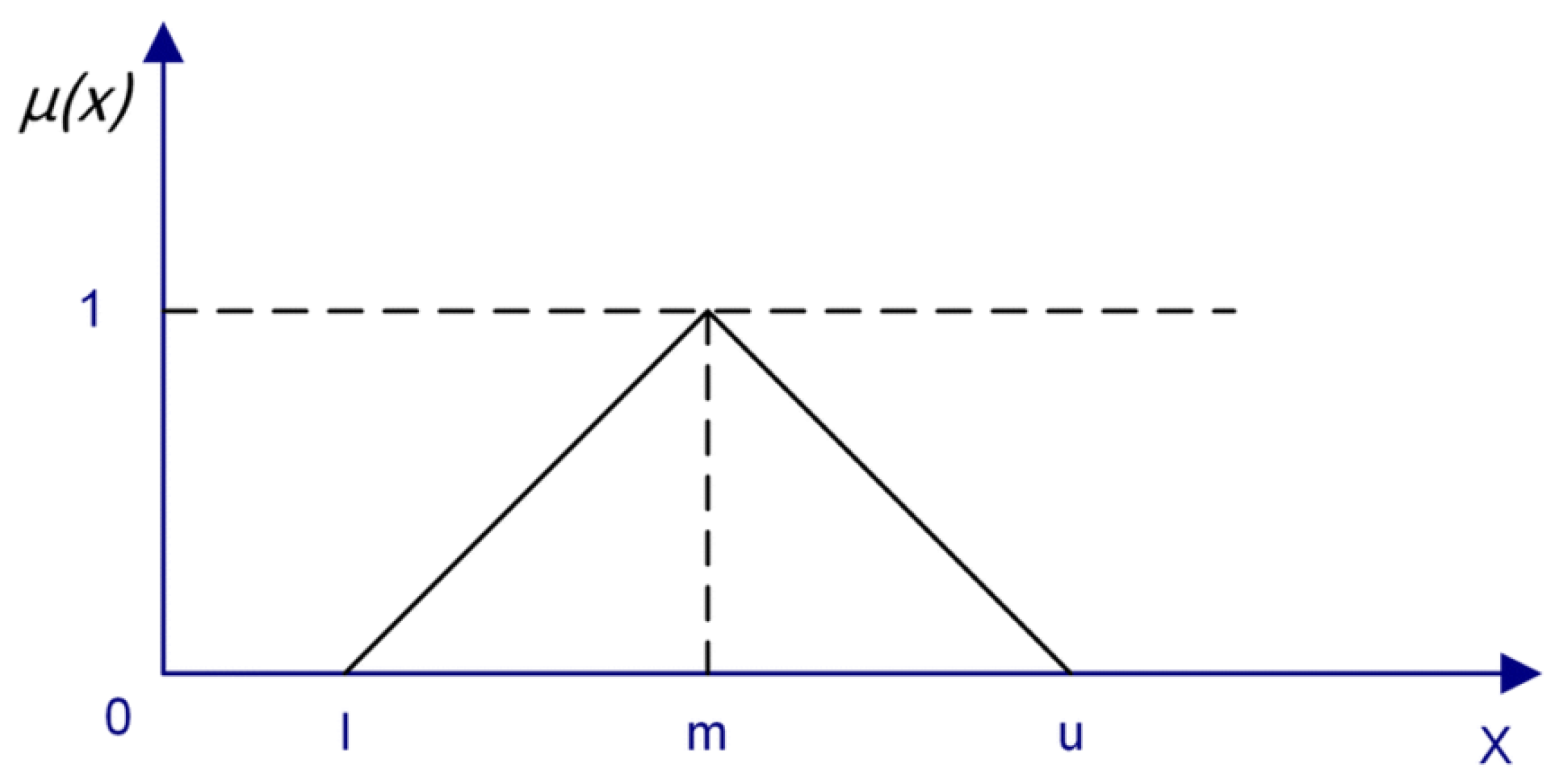
Fuzzy numbers are usually represented by triangular fuzzy numbers (TFN), trapezoidal or Gaussian fuzzy numbers [49]. According to numerous definitions [50]. The triangular fuzzy number à is represented as à = (l,m,u) where its membership function $x\in \tilde{A} , {\mu }_{\tilde{A}}\left(x\right):ℝ\to \left[0,1\right]$ is given by Equation (1) and shown in Figure 1:

$${\mu }_{\tilde{A}} \left(x\right)=\{\begin{array}{c}0 x<l\\ \begin{array}{cc}\frac{x-l}{m-l}& l\le x\le m\end{array}\\ \begin{array}{cc}\frac{u-x}{u-m}& m\le x\le u\end{array}\\ 0 x>u\end{array}$$

(1)

3.1. Fuzzy TOPSIS Method

The traditional TOPSIS method was originally presented by Hwang and Yoon [51], This method has been widely used and modified by several researchers in numerous fields to deal with different fuzzy numbers [52].

According to the fuzzy TOPSIS method, the optimal alternative is selected if it has the shortest distance to the Fuzzy Positive Ideal Solution and the longest distance from the Fuzzy Negative Ideal Solution. The Fuzzy Positive Ideal Solution includes the best performance values for each alternative whereas the Fuzzy Negative Ideal Solution comprises the worst performance values. The fuzzy TOPSIS method includes the following steps:

Step 1: Forming the fuzzy decision matrix by m alternatives and n criteria (Equation (2)).

Step 2: Normalizing the fuzzy decision matrix (Equation (3)).

Step 3: Constructing the weighted normalized decision matrix (Equation (4)).

Step 4: Identifying the Fuzzy Positive Ideal Solution together with the Fuzzy Negative Ideal Solution (Equation (5)).

Step 5: Determining the Euclidean distance between each alternative and the Fuzzy Positive Ideal Solution as well as the Fuzzy Negative Ideal Solution (Equation (6)).

Step 6: Computing the relative closeness coefficient (Equation (7)).

Step 7: Ranking the alternatives. The best alternative is chosen that has the largest value of closeness coefficient [53].

$$\tilde{X}=\left[\begin{array}{ccc}{\tilde{x}}_{11}& \cdots & {\tilde{x}}_{1n}\\ ⋮& \ddots & ⋮\\ {\tilde{x}}_{m1}& \cdots & {\tilde{x}}_{mn}\end{array}\right]=\left[\begin{array}{ccc}\left({\tilde{x}}_{11}^l,{\tilde{x}}_{11}^m,{\tilde{x}}_{11}^u\right)& \cdots & \left({\tilde{x}}_{1n}^l,{\tilde{x}}_{1n}^m,{\tilde{x}}_{1n}^u\right)\\ ⋮& \ddots & ⋮\\ \left({\tilde{x}}_{m1}^l,{\tilde{x}}_{m1}^m,{\tilde{x}}_{m1}^u\right)& \cdots & \left({\tilde{x}}_{mn}^l,{\tilde{x}}_{mn}^m,{\tilde{x}}_{mn}^u\right)\end{array}\right]$$

(2)

$${\tilde{X}}^N=\left[{\tilde{x}}_{ij}^N\right],\hspace{1em} {\tilde{x}}_{ij}^N=\{\begin{array}{c}\frac{{\tilde{x}}_{ij}}{ma{x}_i {\tilde{x}}_{ij}^u} Positive Criteria\\ \frac{mi{n}_i {\tilde{x}}_{ij}^l}{{\tilde{x}}_{ij}} Negative Criteria\end{array}$$

(3)

$${\tilde{V}}^N=\left[{\tilde{V}}_{ij}^N\right], {\tilde{V}}_{ij}^N={\tilde{x}}_{ij}^N\ast {\tilde{w}}_j$$

(4)

$$\begin{gathered} {\tilde{V}}^{+}=\left({\tilde{V}}_1^{+},{\tilde{V}}_2^{+},\dots ,{\tilde{V}}_n^{+}\right)=\left(ma{x}_i{\tilde{V}}_{i1}^N,ma{x}_i{\tilde{V}}_{i2}^N,\dots ,ma{x}_i{\tilde{V}}_{in}^N\right) \\ {\tilde{V}}^{-}=\left({\tilde{V}}_1^{-},{\tilde{V}}_2^{-},\dots ,{\tilde{V}}_n^{-}\right)=\left(mi{n}_i{\tilde{V}}_{i1}^N,mi{n}_i{\tilde{V}}_{i2}^N,\dots ,mi{n}_i{\tilde{V}}_{in}^N\right) \end{gathered}$$

(5)

$$\begin{gathered} d_i^{+}={\sum }_{j=1}^n{d}_{\nu }\left({\tilde{V}}_{ij}^N,{\tilde{V}}_j^{+}\right) , d_i^{-}={\sum }_{j=1}^n{d}_{\nu }\left({\tilde{V}}_{ij}^N,{\tilde{V}}_j^{-}\right) \\ {d}_{\nu }\left({\tilde{A}}_1,{\tilde{A}}_2\right)=\sqrt{\frac{1}{3} \left[{\left(l_1-l_2\right)}^2+{\left(m_1-m_2\right)}^2+{\left(u_1-u_2\right)}^2\right]} \end{gathered}$$

(6)

$$C_i=\frac{d_i^{-}}{d_i^{+}+d_i^{-}}$$

(7)

3.2. Fuzzy SWARA Method

The SWARA (Stepwise Weight Assessment Ratio Analysis) method was first introduced by Kersuliene et al. [54], to estimate the criteria weights considering decision-makers’ preferences. The fuzzy SWARA method determines the importance weights of criteria through the following process which is similar to the fuzzy TOPSIS method [55,56]:

Step 1: Sorting the criteria in descending order in terms of their expected importance, i.e., the most important criterion is ranked first, and the least important criterion is ranked last.

Step 2: Determining the relative importance of each criterion: each of k decision-makers (experts) expresses the relative significance of criterion j in relation to the previous criterion j-1 (for all given criteria) in order to determine the sj ratio which is called the Comparative importance of average value [54]. The fuzzy comparison scale shown in

Table 2. The fuzzy comparison scale for the assessment of evaluation criteria [55].

Linguistic Variable	Response Scale
Equally important	(1, 1, 1)
Moderately less important	(2/3, 1, 3/2)
Less important	(2/5, 1/2, 2/3)
Very less important	(2/7, 1/3, 2/5)
Much less important	(2/9, 1/4, 2/7)

is used. The summation of the mean values of experts’ opinions is obtained for evaluating criteria, employing the minimum, arithmetic mean, and maximum values of the corresponding scores (Equation (8)).

Step 3: Obtaining the coefficient (Equation (9)).

Step 4: Obtaining the fuzzy recalculated weights (Equation (10)).

Step 5: Calculating the ultimate relative fuzzy weight of each criterion j (Equation (11)).

$${\tilde{s}}_j=\left({\tilde{s}}_{jl},{\tilde{s}}_{jm},{\tilde{s}}_{ju}\right)=(\min {\tilde{s}}_{jlk},\frac{{{\displaystyle \sum }}_{k=1}^K{\tilde{s}}_{jmk}}{K},\max {\tilde{s}}_{juk})$$

(8)

$${\tilde{k}}_j=\{\begin{array}{c}\tilde{1} j=1\\ {\tilde{s}}_j+\tilde{1} j>1\end{array}$$

(9)

$${\tilde{q}}_j=\{\begin{array}{c}\tilde{1} j=1\\ \frac{{\tilde{x}}_{j-1}}{{\tilde{k}}_j} j>1\end{array}$$

(10)

$${\tilde{w}}_j=\frac{{\tilde{q}}_j}{{{\displaystyle \sum }}_{k=1}^n{\tilde{q}}_k} ,\hspace{1em}{\tilde{w}}_j=\left({\tilde{w}}_{jl},{\tilde{w}}_{jm},{\tilde{w}}_{ju}\right)$$

(11)

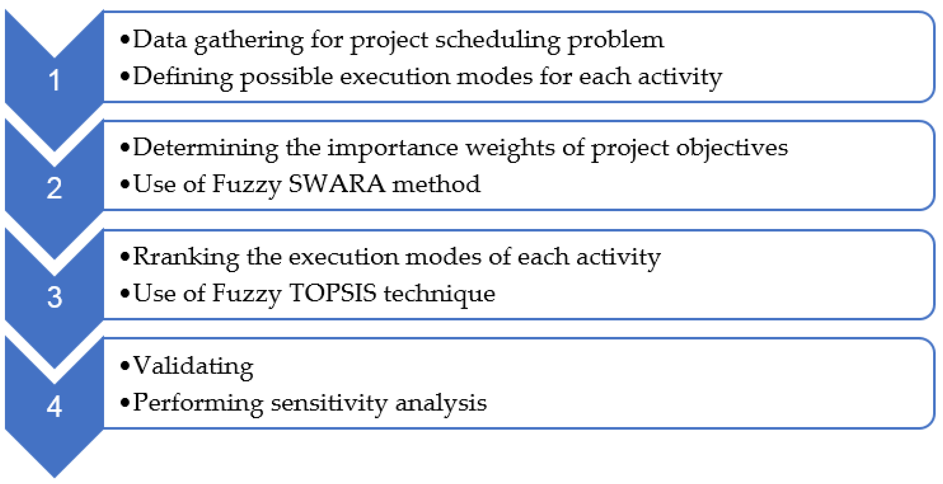
The steps of the research methodology is displayed in Figure 2.

4. Results and Discussion

4.1. Case Studies

In this section, the proposed approach was implemented on a subproject of a large-size project comprising feasibility studies, design and engineering, construction and installation, inspection, and commissioning of an oil and gas field development. The subproject is presented due to the ease of calculations and the proposed method can be applied to the entire project and other large-sized projects. This subproject includes 18 activities, each of which can be executed in seven modes. This project can be performed in 7¹⁸ different combinations of activity execution modes. In this study, the best activity execution modes of these numerous combinations are found by using the MCDM approach. 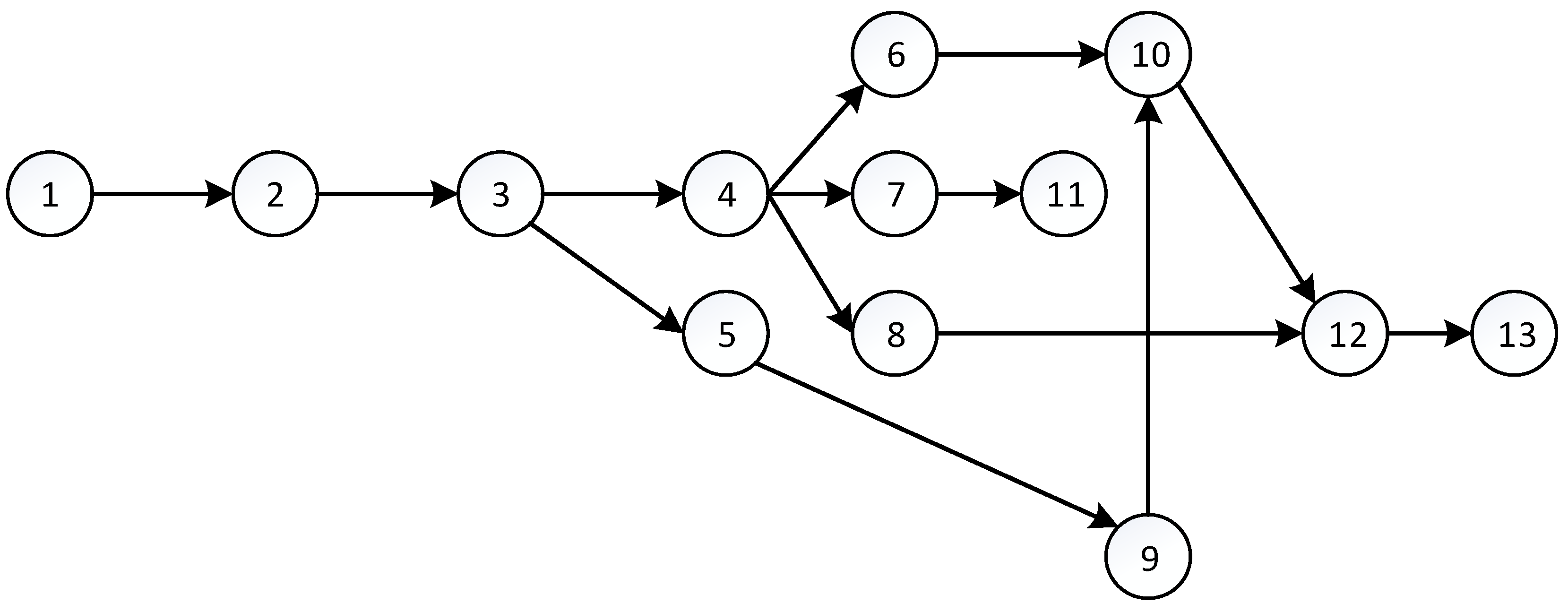Figure 3 shows the activity network of the project.

Given that each activity can be performed in seven execution modes, the amounts of duration, cost, and quality corresponding with various activity execution modes are represented in Appendix A. The activity duration and cost were estimated based on pessimistic, most likely, and optimistic scenarios through historical documents and expert judgment. The five-point Likert scale (very low, low, medium, high, and very high) was used for the quality factor based on different combinations of duration and cost. Finally, the execution modes of the activities are defined regarding the three main project goals including cost, time, and quality.

The fuzzy SWARA method was employed to calculate the weights of project objectives (criteria) including time, cost, and quality. Experts were asked to rank goals from highest to lowest. The importance weight is obtained according to Table 2. The first criterion has no relative importance and from the second criterion onwards, each criterion is weighed against the previous criterion.

Table 3. Experts’ opinions using the SWARA method.

Expert	Time to Cost			Quality to Time
E1	1	1	1	0.4	0.5	0.667
E2	0.667	1	1.5	0.667	1	1.5
E3	0.4	0.5	0.667	1	1	1
E4	0.4	0.5	0.667	0.667	1.000	1.5
E5	1	1	1	0.4	0.5	0.667
E6	0.4	0.5	0.667	1	1	1.000

shows the opinions of experts for ranking time, cost and quality objectives.

Then, the weight of each goal is obtained using the Equations (8)–(11). The final results are shown in

Table 4. Criteria weights obtained using the SWARA method.

	$\widetilde{{\mathit{s}}_{\mathit{j}}}$			$\widetilde{{\mathit{k}}_{\mathit{j}}}$			$\widetilde{{\mathit{q}}_{\mathit{j}}}$			$\widetilde{{\mathit{w}}_{\mathit{j}}}$
Cost	-	-	-	1	1	1	1	1	1	0.64	0.53	0.45
Time	1.5	0.75	0.40	2.50	1.75	1.40	0.714	0.571	0.4	0.32	0.30	0.26
Quality	1.5	0.83	0.40	2.50	1.83	1.40	0.51	0.311	0.16	0.23	0.17	0.10

.

After determining the weights of time, cost, and quality objectives shown in Table 4, the executive modes of each activity were ordered and ranked using the fuzzy TOPSIS technique. The results are shown in Appendix B.

According to

Table 5. Results of the project (project by 13 activities).

	Time			Cost ($)			Quality
	L	M	U	L	M	U	L	M	U
Total Project	508	564	594	260,883	289,872	304,835	0.615	0.760	0.960

, this project is implemented with a duration of 564 days, costs of USD 289,872, and quality level of 0.760, obtained based on α = 1 through the alpha-cut defuzzification method.

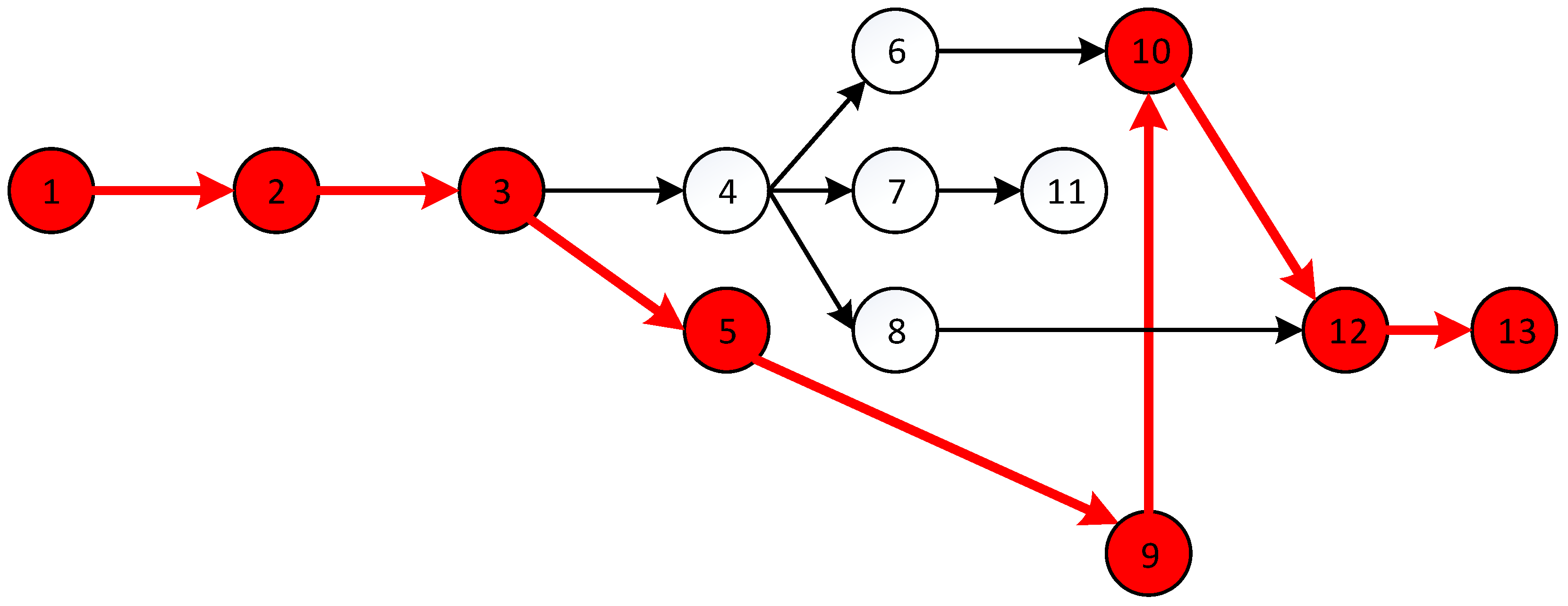
According to Appendix B and

Table 6. Results of fuzzy TOPSIS (project by 32 activities).

N	Execution Modes (First Rank)	d+	d−	C	N	Execution Modes (First Rank)	d+	d−	C
1	M2	0.006938	0.031806	0.8209	17	M3	0.000458	0.027914	0.9839
2	M3	0.000501	0.023149	0.9788	18	M3	0.007049	0.041618	0.8552
3	M2	0.002115	0.033227	0.9402	19	M2	0.002676	0.019518	0.8794
4	M3	0.002658	0.022258	0.8933	20	M4	0.008447	0.032412	0.7933
5	M3	0.000492	0.030102	0.9839	21	M5	0.000869	0.012584	0.9354
6	M3	0.007039	0.034045	0.8287	22	M1	0.002408	0.015698	0.8670
7	M2	0.006581	0.032499	0.8316	23	M1	0.00118	0.012404	0.9132
8	M3	0.000463	0.027914	0.9837	24	M2	0.005123	0.010047	0.6623
9	M2	0.004299	0.030724	0.8772	25	M2	0.005123	0.010047	0.6623
10	M3	0.002931	0.022287	0.8838	26	M2	0.003374	0.019504	0.8525
11	M4	0.000246	0.140369	0.9983	27	M4	0.008734	0.032385	0.7876
12	M3	0.007022	0.039533	0.8492	28	M4	0.00305	0.008765	0.7419
13	M2	0.006475	0.035878	0.8471	29	M1	0.002411	0.015698	0.8669
14	M3	0.000468	0.032043	0.9856	30	M1	0.001182	0.012404	0.9130
15	M2	0.002106	0.032087	0.9384	31	M2	0.005079	0.012404	0.7095
16	M3	0.003014	0.019972	0.8689	32	M2	0.005079	0.012404	0.7095

, each activity’s execution mode with the highest rank was determined and selected for implementation. The total duration of the project was calculated based on the critical path of the project (Figure 4), total project costs were obtained from the sum of activity costs, and the quality of the project was computed based on the geometric mean of the quality of each activity. The results are shown in

Table 7. Results of the project (project by 32 activities).

	Time			Cost ($)			Quality
	L	M	U	L	M	U	L	M	U
Total Project	228	266	304	71,328.5	83,916	96,503.6	68	80	92.1

.

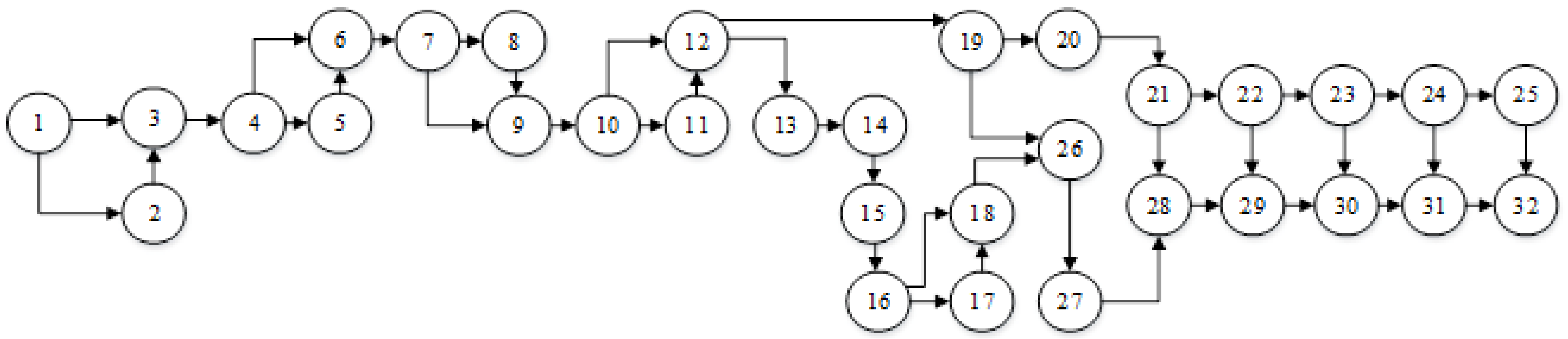
To show the effectiveness of the proposed model, the model was implemented on another construction project with 32 activities. The project network and project data are displayed in Figure 5 and Appendix C, respectively. It should be noted that the total number of different combinations of project implementation based on the presented activity execution modes is 28 * 55 * 819.

According to Table 7, this project is implemented with a duration of 266 days, costs of $83,916, and quality level of 80%, obtained based on α = 1 through the alpha-cut defuzzification method.

4.2. Sensitivity Analysis

Two points have been considered in ranking the different execution modes of each activity using the fuzzy TOPSIS method. The first point is the negativity of time and cost and the positiveness of quality. The second point is that the importance weights of three objectives (criteria) have been determined by the SWARA method based on the opinions of experts in the field of civil engineering and project management. First, the time objective is considered as the most important project goal, and the activities are executed in the modes with the shortest durations, the execution modes of 6 and 7 of all activities have the minimum durations. Then, the cost objective is considered as the most important objective in the project, and the activities are executed in the modes with the lowest costs. Finally, the quality objective is considered as the most important project objective, and the activities are executed in the modes with the highest quality. The findings are displayed in

Table 8. Sensitivity analysis (project by 13 activities).

		Time			Cost			Quality
		L	M	U	L	M	U	L	M	U
Total Project		508	564	594	260,883	289,872	304,835	0.615	0.760	0.960
Min Time	Min Time & Min Cost	463	513	542	255,896	284,333	299,296	0.416	0.612	0.815
	Min Time & Max Quality				257,870	286,525	301,490	0.450	0.644	0.847
Min Cost	Min Cost & Min T	513	570	600	230,308	255,896	269367	0.416	0.612	0.815
	Min Cost & Max Q	523	581	611				0.527	0.715	0.915
Max Q	Max Q & Min T	508	564	594	255,348	283,723	298,655	0.648	0.776	0.976
	Max Q & Min C	514	571	601	242,245	269,161	283,328

.

Table 6 shows the rankings of activity execution modes obtained by the fuzzy TOPSIS method. The total project duration was calculated using the critical path method, the total project cost was equal to the summation of activity costs and the project quality was determined based on the geometric average quality of each activity.

Table 9. Sensitivity analysis (project by 32 activities).

		Time			Cost			Quality
		L	M	U	L	M	U	L	M	U
Total Project		228	266	304	71,328.5	83,916	96,503.6	68.0	80.0	92.1
Min Time	Min Time & Min Cost	83	105	129	78,891	91,290.8	104,082.8	73.0	84.6	96.4
	Min Time & Max Quality				79,218.0	91,675.0	104,524.5	73.2	84.8	96.6
Min Cost	Min Cost & Min Time	289	338	387	64,914.9	76,370.5	87,826.1	66.6	78.3	90.1
	Min Cost & Max Q	289	338	387				66.6	78.3	90.1
Max Q	Max Q & Min Time	85	107	131	79,066.4	91,496.6	104,319.3	73.6	84.8	96.6
	Max Q & Min Cost	135	163	190	77,566.8	90,570.4	102,735.2

displays the findings.

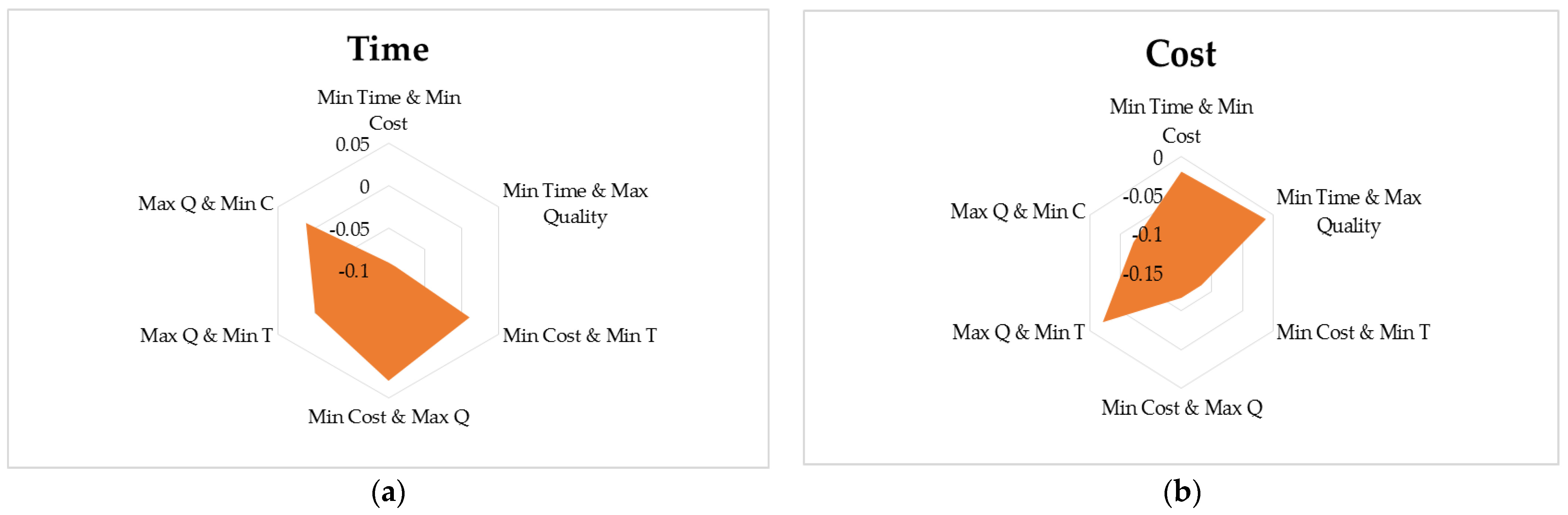
Comparing the activity execution modes with the shortest durations to the results obtained from the fuzzy TOPSIS method shows that the two objectives of time and cost have improved significantly, but the quality objective has diminished. In addition, the selection of activity execution modes with the lowest costs results in the worse values of time and quality objectives. Also, the selection of activity execution modes with the highest quality levels results in increasing the value of time objective and decreasing the value of cost objective (Max Q and Min C). Figure 6 shows the percentage of change of each method in α-cut of 1 (the value of m in à = (l, m, u)).

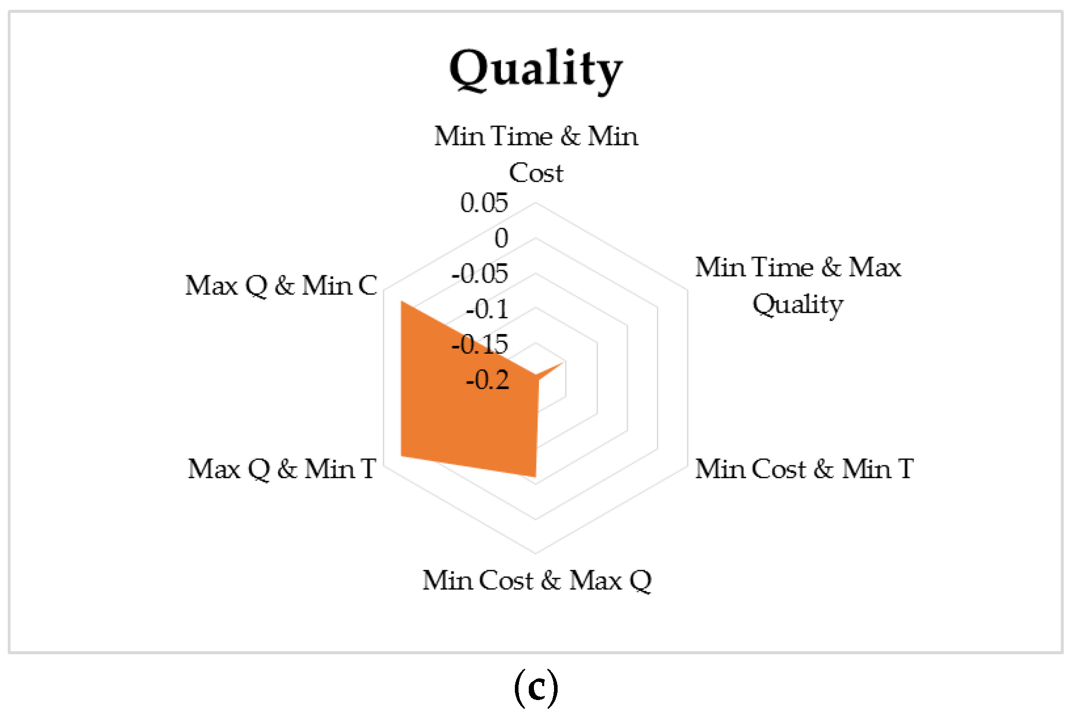
Figure 6 shows the percentage of changes in different modes based on the numbers obtained for the whole project. Figure 6a shows the percentage of changes in the rows of Table 8 based on the factor of total project duration, Figure 6b shows the percentage of changes in the rows of Table 8 based on the factor of total project cost, and Figure 6c shows the percentage of changes in the rows of Table 8 based on the factor of project quality.

Same as the first example (project with 13 activities), the sensitivity analysis was conducted for the second project with 32 activities. The results are presented in Table 9.

As shown in Table 9, a comparison of the shortest duration method with the results obtained from the fuzzy TOPSIS method demonstrates that time and quality have improved significantly but cost has deteriorated. Also, time and quality have deteriorated in the project implementation with the lowest cost method, and time and cost have worsened in the project implementation with the highest quality level.

4.3. Practical Implications

The project iron triangle including time, cost, and quality is of significant importance for evaluating construction projects that all project managers seek to optimize these three factors simultaneously so that they can complete the project within the shortest duration, minimum cost, and maximum quality. Each activity in the project can be performed in various execution modes that have different duration, cost, and quality. Project managers must decide on the choice of each execution mode for every activity so that they can ultimately achieve the project goals and objectives. Therefore, in this study, the multi-criteria decision-making approaches have been used to trade off among project objectives. The selection of any execution mode for each activity through ranking the execution modes can finally accomplish the project with the best trade-off values of three objectives that can be expressed as one of the most significant managerial and practical implications of this study.

5. Conclusions

Accurate estimation of completion time, implementation cost, and acceptable quality level of a project is one of the most serious challenges in project management. A project is successfully accomplished if it is finished in the shortest makespan and lowest costs along with the highest quality in accordance with what is defined within the project scope. Project managers should develop a schedule according to the uncertainty in the environment, conditions, and restrictions of the project. Quite often it is to reduce the durations of some activities at additional costs so that the project completion is accelerated. Changes in the duration and cost of each activity also have a great impact on quality. Therefore, the balance of time, cost, and quality has been attracted more attention from project practitioners. A review of the methods used by other researchers in the field of project scheduling revealed that previous models seldom considered uncertainty conditions for all three project goals of time, cost, and quality. On the other hand, previous studies have considered the project goals with equal importance. In this study, this significant problem was investigated in construction projects. The best execution mode of each activity was selected using the fuzzy MCDM approach taking the three substantial project goals and objectives of time, cost, and quality into consideration. First, the importance weights of the time, cost, and quality objectives were identified by experts using the fuzzy SWARA technique. Then, each activity execution mode, which has a different duration, cost, and quality, was ordered and ranked through the fuzzy TOPSIS technique. Finally, the execution method of each activity with the highest rank was considered as the best execution mode of that activity and the project schedule was developed based on these execution modes.

The obtained results in both case studies showed that the best execution mode selected for each activity is between the desired values of the objective functions so that the duration of the selected executive method is close to the most likely activity duration. The situation is more favorable for the cost objective function than for the time objective function. The reason is that the weight of the cost objective function is higher than other goals, and the weight of the quality objective function is lower than others. However, the importance weights of the project goals may be changed based on the opinions of the project stakeholders.

The results showed a significant improvement in the project objectives comparing to different activity execution modes including the least duration, the lowest cost, and the highest quality level of each activity execution. In the sensitivity analysis section, the percentage of changes in each of the project objectives compared to other different modes in the entire project was analyzed which showed a high improvement in the results.

Given that the problem of minimizing project duration and cost together with maximizing project quality is one of the most important challenges facing project planners and practitioners, the decision-making models were exploited in this research for selecting the best possible activity execution modes. The present study can assist project practitioners and managers with choosing the appropriate activity execution methods for accomplishing the project in the shortest makespan and at the lowest costs together with the most superb quality level.

Lack of enough information along with difficulties associated with estimating the time, cost, and quality of each activity execution mode can be mentioned as the limitations of the current study. The finish-to-start precedence relationship with zero time lag was considered as a basic assumption. Since various execution modes for each activity have been independently ranked, other precedence relationships can be considered. As some suggestions for future research, other types of precedence relationships should be considered in the model. Also, uncertain data such as grey data can be used. Moreover, other decision-making methods may be applied and the results be compared with the methods proposed in this study.

References

- Afshar, A.; Ziaraty, A.K.; Kaveh, A.; Sharifi, F. Nondominated archiving multicolony ant algorithm in time–cost trade-off optimization. J. Constr. Eng. Manag. 2009, 135, 668–674. [Google Scholar] [CrossRef]
- Hafezalkotob, A.; Hosseinpour, E.; Moradi, M.; Khalili-Damghani, K. Multi-resource trade-off problem of the project contractors in a cooperative environment: Highway construction case study. Int. J. Manag. Sci. Eng. Manag. 2018, 13, 129–138. [Google Scholar] [CrossRef]
- Babu, A.J.G.; Suresh, N. Project management with time, cost, and quality considerations. Eur. J. Oper. Res. 1996, 88, 320–327. [Google Scholar] [CrossRef]
- Khang, D.B.; Myint, Y.M. Time, cost and quality trade-off in project management: A case study. Int. J. Proj. Manag. 1999, 17, 249–256. [Google Scholar] [CrossRef]
- Kim, J.; Kang, C.; Hwang, I. A practical approach to project scheduling: Considering the potential quality loss cost in the time–cost tradeoff problem. Int. J. Proj. Manag. 2012, 30, 264–272. [Google Scholar] [CrossRef]
- Saif, A.; Abbas, S.; Fayed, Z. The PDBO algorithm for discrete time, cost and quality trade-off in software projects with expressing quality by defects. Procedia Comput. Sci. 2015, 65, 930–939. [Google Scholar] [CrossRef] [Green Version]
- Derbe, G.; Li, Y.; Wu, D.; Zhao, Q. Scientometric review of construction project schedule studies: Trends, gaps and potential research areas. J. Civ. Eng. Manag. 2020, 26, 343–363. [Google Scholar] [CrossRef] [Green Version]
- Moghadam, E.K.; Sharifi, M.; Rafiee, S.; Chang, Y.K. Time–Cost–Quality Trade-Off in a Broiler Production Project Using Meta-Heuristic Algorithms: A Case Study. Agriculture 2020, 10, 3. [Google Scholar] [CrossRef] [Green Version]
- Antucheviciene, J.; Kala, Z.; Marzouk, M.; Vaidogas, E.R. Decision making methods and applications in civil engineering. Math. Probl. Eng. 2015, 2015. [Google Scholar] [CrossRef]
- Balali, A.; Moehler, R.C.; Valipour, A. Ranking cost overrun factors in the mega hospital construction projects using Delphi-SWARA method: An Iranian case study. Int. J. Constr. Manag. 2020, 1–9. [Google Scholar] [CrossRef]
- Khalesi, H.; Balali, A.; Valipour, A.; Antucheviciene, J.; Migilinskas, D.; Zigmund, V. Application of Hybrid SWARA–BIM in Reducing Reworks of Building Construction Projects from the Perspective of Time. Sustainability 2020, 12, 8927. [Google Scholar] [CrossRef]
- Li, H.; Wang, W.; Fan, L.; Li, Q.; Chen, X. A novel hybrid MCDM model for machine tool selection using fuzzy DEMATEL, entropy weighting and later defuzzification VIKOR. Appl. Soft Comput. 2020, 91, 106207. [Google Scholar] [CrossRef]
- Koulinas, G.K.; Xanthopoulos, A.S.; Tsilipiras, T.T.; Koulouriotis, D.E. Schedule Delay Risk Analysis in Construction Projects with a Simulation-Based Expert System. Buildings 2020, 10, 134. [Google Scholar] [CrossRef]
- Abdellatif, H.; Alshibani, A. Major Factors Causing Delay in the Delivery of Manufacturing and Building Projects in Saudi Arabia. Buildings 2019, 9, 93. [Google Scholar] [CrossRef] [Green Version]
- Moselhi, O. Schedule compression using the direct stiffness method. Can. J. Civ. Eng. 1993, 20, 65–72. [Google Scholar] [CrossRef]
- Manzoor, B.; Othman, I.; Gardezi, S.S.S.; Harirchian, E. Strategies for Adopting Building Information Modeling (BIM) in Sustainable Building Projects—A Case of Malaysia. Buildings 2021, 11, 249. [Google Scholar] [CrossRef]
- Harirchian, E.; Lahmer, T. Developing a hierarchical type-2 fuzzy logic model to improve rapid evaluation of earthquake hazard safety of existing buildings. Structures 2020, 28, 1384–1399. [Google Scholar] [CrossRef]
- Liu, L.; Burns, S.A.; Feng, C.W. Construction time-cost trade-off analysis using LP/IP hybrid method. J. Constr. Eng. Manag. 1995, 121, 446–454. [Google Scholar] [CrossRef]
- Demeulemeester, E.; De Reyck, B.; Foubert, B.; Herroelen, W.; Vanhoucke, M. New computational results on the discrete time/cost trade-off problem in project networks. J. Oper. Res. Soc. 1998, 49, 1153–1163. [Google Scholar] [CrossRef]
- Vanhoucke, M. New computational results for the discrete time/cost trade-off problem with time-switch constraints. Eur. J. Oper. Res. 2005, 165, 359–374. [Google Scholar] [CrossRef]
- El-Rayes, K.; Kandil, A. Time-cost-quality trade-off analysis for highway construction. J. Constr. Eng. Manag. 2005, 131, 477–486. [Google Scholar] [CrossRef]
- Tareghian, H.R.; Taheri, S.H. On the discrete time, cost and quality trade-off problem. Appl. Math. Comput. 2006, 181, 1305–1312. [Google Scholar] [CrossRef]
- Zhang, H.; Xing, F. Fuzzy-multi-objective particle swarm optimization for time–cost–quality tradeoff in construction. Autom. Constr. 2010, 19, 1067–1075. [Google Scholar] [CrossRef]
- Harirchian, E.; Jadhav, K.; Mohammad, K.; Aghakouchaki Hosseini, S.E.; Lahmer, T. A comparative study of MCDM methods integrated with rapid visual seismic vulnerability assessment of existing RC structures. Appl. Sci. 2020, 10, 6411. [Google Scholar] [CrossRef]
- Chen, H.; Li, X.Y.; Lu, X.R.; Sheng, N.; Zhou, W.; Geng, H.P.; Yu, S. A multi-objective optimization approach for the selection of overseas oil projects. Comput. Ind. Eng. 2020, 151, 106977. [Google Scholar] [CrossRef]
- Ma, J.; Harstvedt, J.D.; Jaradat, R.; Smith, B. Sustainability driven multi-criteria project portfolio selection under uncertain decision-making environment. Comput. Ind. Eng. 2020, 140, 106236. [Google Scholar] [CrossRef]
- Tavana, M.; Khosrojerdi, G.; Mina, H.; Rahman, A. A new dynamic two-stage mathematical programming model under uncertainty for project evaluation and selection. Comput. Ind. Eng. 2020, 149, 106795. [Google Scholar] [CrossRef]
- Issa, U.H.; Miky, Y.H.; Abdel-Malak, F.F. A decision support model for civil engineering projects based on multi-criteria and various data. J. Civ. Eng. Manag. 2019, 25, 100–113. [Google Scholar] [CrossRef]
- Walczak, D.; Rutkowska, A. Project rankings for participatory budget based on the fuzzy TOPSIS method. Eur. J. Oper. Res. 2017, 260, 706–714. [Google Scholar] [CrossRef]
- Mandic, D.; Jovanovic, P.; Bugarinovic, M. Two-phase model for multi-criteria project ranking: Serbian Railways case study. Transp. Policy 2014, 36, 88–104. [Google Scholar] [CrossRef]
- Valipour, A.; Yahaya, N.; Md Noor, N.; Antuchevičienė, J.; Tamošaitienė, J. Hybrid SWARA-COPRAS method for risk assessment in deep foundation excavation project: An Iranian case study. J. Civ. Eng. Manag. 2017, 23, 524–532. [Google Scholar] [CrossRef] [Green Version]
- Mota, A.; Ávila, P.; Albuquerque, R.; Costa, L.; Bastos, J. A Framework for Time-Cost-Quality Optimization in Project Management Problems Using an Exploratory Grid Concept in the Multi-Objective Simulated-Annealing. Int. J. Inf. Technol. Decision Mak. 2021, 20, 1095–1120. [Google Scholar] [CrossRef]
- Nguyen, D.T.; Le-Hoai, L.; Tarigan, P.B.; Tran, D.H. Tradeoff time cost quality in repetitive construction project using fuzzy logic approach and symbiotic organism search algorithm. Alex. Eng. J. 2021. [Google Scholar] [CrossRef]
- Abbasi, D.; Ashrafi, M.; Ghodsypour, S.H. A multi objective-BSC model for new product development project portfolio selection. Expert Syst. Appl. 2020, 162, 113757. [Google Scholar] [CrossRef]
- Banihashemi, S.A.; Khalilzadeh, M.; Shahraki, A.; Malkhalifeh, M.R.; Ahmadizadeh, S.S.R. Optimization of environmental impacts of construction projects: A time–cost–quality trade-off approach. Int. J. Environ. Sci. Technol. 2020, 18, 631–646. [Google Scholar] [CrossRef]
- Banihashemi, S.A.; Khalilzadeh, M. Time-cost-quality-environmental impact trade-off resource-constrained project scheduling problem with DEA approach. Eng. Constr. Arch. Manag. 2020, 28, 1979–2004. [Google Scholar] [CrossRef]
- Karbassi Yazdi, A.; Komijan, A.R.; Wanke, P.F.; Sardar, S. Oil project selection in Iran: A hybrid MADM approach in an uncertain environment. Appl. Soft Comput. 2020, 88, 106066. [Google Scholar] [CrossRef]
- Liu, D.; Li, H.; Wang, H.; Qi, C.; Rose, T. Discrete symbiotic organisms search method for solving large-scale time-cost trade-off problem in construction scheduling. Expert Syst. Appl. 2020, 148, 113230. [Google Scholar] [CrossRef]
- RezaHoseini, A.; Ghannadpour, S.F.; Hemmati, M. A comprehensive mathematical model for resource-constrained multi-objective project portfolio selection and scheduling considering sustainability and projects splitting. J. Clean. Prod. 2020, 269, 122073. [Google Scholar] [CrossRef]
- Aouam, T.; Vanhoucke, M. An agency perspective for multi-mode project scheduling with time/cost trade-offs. Comput. Oper. Res. 2019, 105, 167–186. [Google Scholar] [CrossRef]
- Toloo, M.; Mirbolouki, M. A new project selection method using data envelopment analysis. Comput. Ind. Eng. 2019, 138, 106119. [Google Scholar] [CrossRef]
- Durmuşoğlu, Z.D.U. Assessment of techno-entrepreneurship projects by using Analytical Hierarchy Process (AHP). Technol. Soc. 2018, 54, 41–46. [Google Scholar] [CrossRef]
- Jafarzadeh, H.; Akbari, P.; Abedin, B. A methodology for project portfolio selection under criteria prioritisation, uncertainty and projects interdependency–combination of fuzzy QFD and DEA. Expert Syst. Appl. 2018, 110, 237–249. [Google Scholar] [CrossRef]
- Zolfani, S.H.; Pourhossein, M.; Yazdani, M.; Zavadskas, E.K. Evaluating construction projects of hotels based on environmental sustainability with MCDM framework. Alex. Eng. J. 2018, 57, 357–365. [Google Scholar] [CrossRef]
- Tavana, M.; Abtahi, A.R.; Khalili-Damghani, K. A new multi-objective multi-mode model for solving preemptive time–cost–quality trade-off project scheduling problems. Expert Syst. Appl. 2014, 41, 1830–1846. [Google Scholar] [CrossRef]
- Taylan, O.; Bafail, A.O.; Abdulaal, R.M.; Kabli, M.R. Construction projects selection and risk assessment by fuzzy AHP and fuzzy TOPSIS methodologies. Appl. Soft Comput. 2014, 17, 105–116. [Google Scholar] [CrossRef]
- Chen, S.P.; Tsai, M.J. Time–cost trade-off analysis of project networks in fuzzy environments. Eur. J. Oper. Res. 2011, 212, 386–397. [Google Scholar] [CrossRef]
- Zadeh, L.A. Fuzzy sets. Inf. Control 1965, 8, 338–353. [Google Scholar] [CrossRef] [Green Version]
- Stević, Ž.; Vasiljević, M.; Puška, A.; Tanackov, I.; Junevičius, R.; Vesković, S. Evaluation of suppliers under uncertainty: A multiphase approach based on fuzzy AHP and fuzzy EDAS. Transport 2019, 34, 52–66. [Google Scholar] [CrossRef] [Green Version]
- Van Laarhoven, P.J.; Pedrycz, W. A fuzzy extension of Saaty’s priority theory. Fuzzy Sets Syst. 1983, 11, 229–241. [Google Scholar] [CrossRef]
- Hwang, C.L.; Yoon, K. Multiple Attribute Decision Making Methods and Applications; Springer: Berlin/Heidelberg, Germany, 1981. [Google Scholar]
- Wang, Y.J.; Lee, H.S.; Lin, K. Fuzzy TOPSIS for multi-criteria decision-making. Int. Math. J. 2003, 3, 367–379. [Google Scholar]
- Petrović, G.; Mihajlović, J.; Ćojbašić, Ž.; Madić, M.; Marinković, D. Comparison of three fuzzy MCDM methods for solving the supplier selection problem. Facta Univ. Ser. Mech. Eng. 2019, 17, 455–469. [Google Scholar] [CrossRef]
- Keršulienė, V.; Zavadskas, E.K.; Turskis, Z. Selection of rational dispute resolution method by applying new step-wise weight assessment ratio analysis (Swara). J. Bus. Econ. Manag. 2010, 11, 243–258. [Google Scholar] [CrossRef]
- Mavi, R.K.; Goh, M.; Zarbakhshnia, N. Sustainable third-party reverse logistic provider selection with fuzzy SWARA and fuzzy MOORA in plastic industry. Int. J. Adv. Manuf. Technol. 2017, 91, 2401–2418. [Google Scholar] [CrossRef]
- Vesković, S.; Stević, Ž.; Stojić, G.; Vasiljević, M.; Milinković, S. Evaluation of the railway management model by using a new integrated model DELPHI-SWARA-MABAC. Decision Mak. Appl. Manag. Eng. 2018, 1, 34–50. [Google Scholar] [CrossRef]