Temporal-Spatial Neighborhood Enhanced Sparse Autoencoder for Nonlinear Dynamic Process Monitoring

Abstract

Data-based process monitoring methods have received tremendous attention in recent years, and modern industrial process data often exhibit dynamic and nonlinear characteristics. Traditional autoencoders, such as stacked denoising autoencoders (SDAEs), have excellent nonlinear feature extraction capabilities, but they ignore the dynamic correlation between sample data. Feature extraction based on manifold learning using spatial or temporal neighbors has been widely used in dynamic process monitoring in recent years, but most of them use linear features and do not take into account the complex nonlinearities of industrial processes. Therefore, a fault detection scheme based on temporal-spatial neighborhood enhanced sparse autoencoder is proposed in this paper. Firstly, it selects the temporal neighborhood and spatial neighborhood of the sample at the current time within the time window with a certain length, the spatial similarity and time serial correlation are used for weighted reconstruction, and the reconstruction combines the current sample as the input of the sparse stack autoencoder (SSAE) to extract the correlation features between the current sample and the neighborhood information. Two statistics are constructed for fault detection. Considering that both types of neighborhood information contain spatial-temporal structural features, Bayesian fusion strategy is used to integrate the two parts of the detection results. Finally, the superiority of the method in this paper is illustrated by a numerical example and the Tennessee Eastman process.

1. Introduction

In the last ten years, the modern process industry has become more complex and large scale, and its requirements for safety performance, product quality and economic benefits have been increasing. In particular, the importance of monitoring the safety and environmental footprint in the process industry has become increasingly prominent. The collection of massive sensor data and low dependence on accurate mathematical models and expert knowledge make the data-driven approach gain more and more attention in academia and industry [1]. Multivariate statistical process monitoring (MSPM), as a widely used method, can extract key features in data for process monitoring [2,3].

The high-dimensional data collected by different sensors can reflect the running status of the process and how to effectively extract feature information has become a key step in fault detection. Principal component analysis (PCA) extracts feature information by maximizing global variance to reduce dimensionality [4], and neighborhood preserving embedding (NPE) is based on manifold learning [5], which reduces dimensionality by keeping the local structure of data points and their neighbors unchanged. As the representatives of multivariate statistical algorithms, they have been widely used in chemical process monitoring. In recent years, fault detection schemes based on global information or local information have developed rapidly. Consider that the sample of industrial processes at different times is not statistically independent, but there is a certain correlation. Ku et al. [6] first proposed Dynamic Principal Component Analysis (DPCA), which uses the PCA to build models by constructing augmented data matrices at current and past times, taking into account the time-series correlation between variables, and improving the fault detection effect. Miao et al. [7] proposed Time Series Extended Neighbor Embedding (TNPE), which uses the nearest time neighborhood in the time window to linearly reconstruct the current sample to extract features that can preserve the timing correlation of the samples. Of course, many scholars consider both global information and local information. Zhang et al. [8] combined Principal Component Analysis (PCA) and Locality Preserving Projections (LPP) to propose a global-local structure analysis model (GLSA) for fault detection, which significantly improves the detection performance. Since then, there have been many similar combined methods [9,10].

However, the actual industrial processes not only have dynamic characteristics but also generally have a complex nonlinear relationship. The method to find the projection matrix to obtain features is more suitable for the process with a linear relationship, such as TNPE and the GLSA. Therefore, we need to consider the nonlinear characteristics of industrial processes further. In recent years, the nonlinear dimension reduction techniques have been improved mainly from the following aspects: (1) PCA, (2) slice inverse regression (SIR), (3) active subspace (AS), (4) manifold learning, and (5) the neural network. Nonlinear extension methods based on slice inverse regression, such as kernel SIR, and extension methods based on active subspace, such as Active Manifolds (AMs), were proposed and showed excellent nonlinear feature extraction ability to achieve the purpose of dimensionality reduction. However, most of their methods need to be used under the supervision of the output variable y, or a hypothetical output model is required. Therefore, they are less used in industrial process fault detection and are more suitable for soft sensing [11,12,13]. The extended methods based on PCA and manifold learning have been widely used in fault detection. In recent years, the deep neural network has also begun to be widely used in industrial process monitoring due to their excellent nonlinear feature extraction capabilities, and even further combined with manifold learning and other methods. Cui et al. [14] proposed an ensemble local kernel principal component analysis (ELKPCA), which took into account the global-local structure information of the data and used kernel functions to deal with nonlinear problems. On the other hand, due to the deep neural network can better extract nonlinear features of high-dimensional data, they have gained significant attention in the field of process monitoring in recent years. Zhao et al. [15] proposed a neighborhood preserving neural network (NPNN) based on NPE, so that the nonlinear features that were extracted from high-dimensional data can still maintain local reconstruction better and greatly improve the fault detection ability of the NPE algorithm. Autoencoders (AE), as one of the representatives of neural networks, is a model that reduces dimensionality and extracts nonlinear features from data by minimizing the reconstruction errors of input and output. Stacked sparse autoencoders (SSAE) can build deep models by stacking multiple AEs to extract deeper and more important features from the data. For dealing with the nonlinear dynamic characteristics of the process, Zhu et al. [16] proposed a recursive stacked denoising autoencoder (RSDAE) to extract nonlinear dynamic features and static features and successfully applied them to fault detection. Compared with the kernel method [17], which requires designing the kernel function artificially, the characteristics of deep neural network automatic learning parameters to extract features make it a popular method to deal with the problem of fault detection in nonlinear processes [18,19].

Due to the complicated nonlinear relationship between industrial process variables, there is also a time-series correlation between samples at different times. Considering the sample at a specific moment, its temporal neighborhood or spatial neighborhood can interact with it, so its neighborhood can be used to assist in fault detection. In this paper, a temporal-spatial neighborhood enhanced sparse stack autoencoder (TS-SSAE) is proposed for dynamic nonlinear process monitoring. In a time window, TS-SSAE finds the spatial neighborhoods of the current sample by k-nearest neighbors algorithm (KNN), and reconstruct the neighborhoods by serial correlation weight with the current time, then combine the current sample as the input of the stack sparse autoencoder. Similarly, for the temporal neighborhood, the spatial similarity to the current sample is chosen as a weight to reconstruct the neighborhoods, and then the current sample is combined as the input of the stack sparse autoencoder. Neighborhood reconstruction improves the separability of samples while achieving smooth denoising. The combination of the current sample and the neighborhood reconstruction as input makes the extracted features contain essential information about the current moment and the neighborhood. If the relationship between the current moment and the neighborhood changes, the extracted features will be different. Then, considering the spatial-temporal characteristics of the two neighborhood information, Bayesian theory is used to integrate the $T^2$ and $SPE$ statistics constructed by the two networks, respectively, for fault detection. Finally, a numerical case and the Tennessee Eastman process benchmark are used to demonstrate the effectiveness of the proposed algorithm.

The rest of the article is organized as follows. Firstly, the structure of SSAE is introduced in Section 2, and the TS-SSAE model is proposed in Section 3. In Section 4, the fault detection scheme based on the TS-SSAE model is described. In Section 5, a neighborhood reconstruction experiment is used to show the reconstruction effect. A numerical case and the Tennessee-Eastman process are used to evaluate the algorithm. In Section 6, some conclusions are listed.

2. Preliminaries

Sparse Stack Autoencoder

The initial goal of the autoencoder (AE) is dimensionality reduction. However, when the hidden layer has more nodes than the input layer, AE will not automatically learn the features of input data. If the sparsity constraint is introduced to the hidden layer on the basis of SAE, an efficient feature representation will be obtained by suppressing the output of most hidden units. Therefore, even if the number of hidden layer units increases, stacked sparse autoencoders (SSAE) still have strong feature expression capabilities [20,21], and the learned high-dimensional sparse features are conducive to fault detection.

Sparsity restriction refers to making neurons inactive most of the time. For example, when the activation function of the hidden unit is sigmoid, the output of the neuron is considered to be active when it is close to 1 and is considered to be inactive when it is close to 0. After the sparsity restriction is added, the cost function of SSAE can be expressed by Equation (1), and its structural diagram is shown in Figure 1. It should be noted that the number of feature layers in Figure 1 is variable.

$$J\left(W,b\right)=\frac{1}{n}{{\displaystyle \sum _{i=1}^n\Vert {\stackrel{⌢}{x}}^{\left(i\right)}-x^{\left(i\right)}\Vert }}_2{}^2+\beta {\displaystyle \sum _{j=1}^{s}KL\left(\rho \Vert {\stackrel{⌢}{\rho }}_j\right)}$$

(1)

In Equation (1), the left part is the reconstruction error of the autoencoder, the right part is the hidden layer sparse constraint. Where $\beta$ is the penalty term for controlling the sparse constraint,$S$ is the number of hidden layer neurons, and $KL\left(\rho \Vert {\stackrel{⌢}{\rho }}_j\right)$ is defined by Equation (2). ${\stackrel{⌢}{\rho }}_j$ represents the average activation of hidden unit j, which is defined by Equation (3). $\rho$ is the sparsity parameter whose value is close to zero, and its value determines the degree of neuron sparsity [22].

$$KL\left(\rho \Vert {\stackrel{⌢}{\rho }}_j\right)=\rho \log \frac{\rho }{\stackrel{⌢}{\rho }}+\left(1-\rho \right)\log \frac{1-\rho }{1-{\stackrel{⌢}{\rho }}_j}$$

(2)

$${\stackrel{⌢}{\rho }}_j=\frac{1}{n}{\displaystyle \sum _{i=1}^n{h}_j\left(W_j{x}^{\left(i\right)}\right)}$$

(3)

Minimizing the right part of Equation (1) will make ${\stackrel{⌢}{\rho }}_j$ and $\rho$ as equal as possible, so that the average activation of hidden units is smaller, to achieve the purpose of sparse hidden layers.

3. Temporal-Spatial Neighborhood Enhanced Sparse Stack Autoencoder (TS-SSAE)

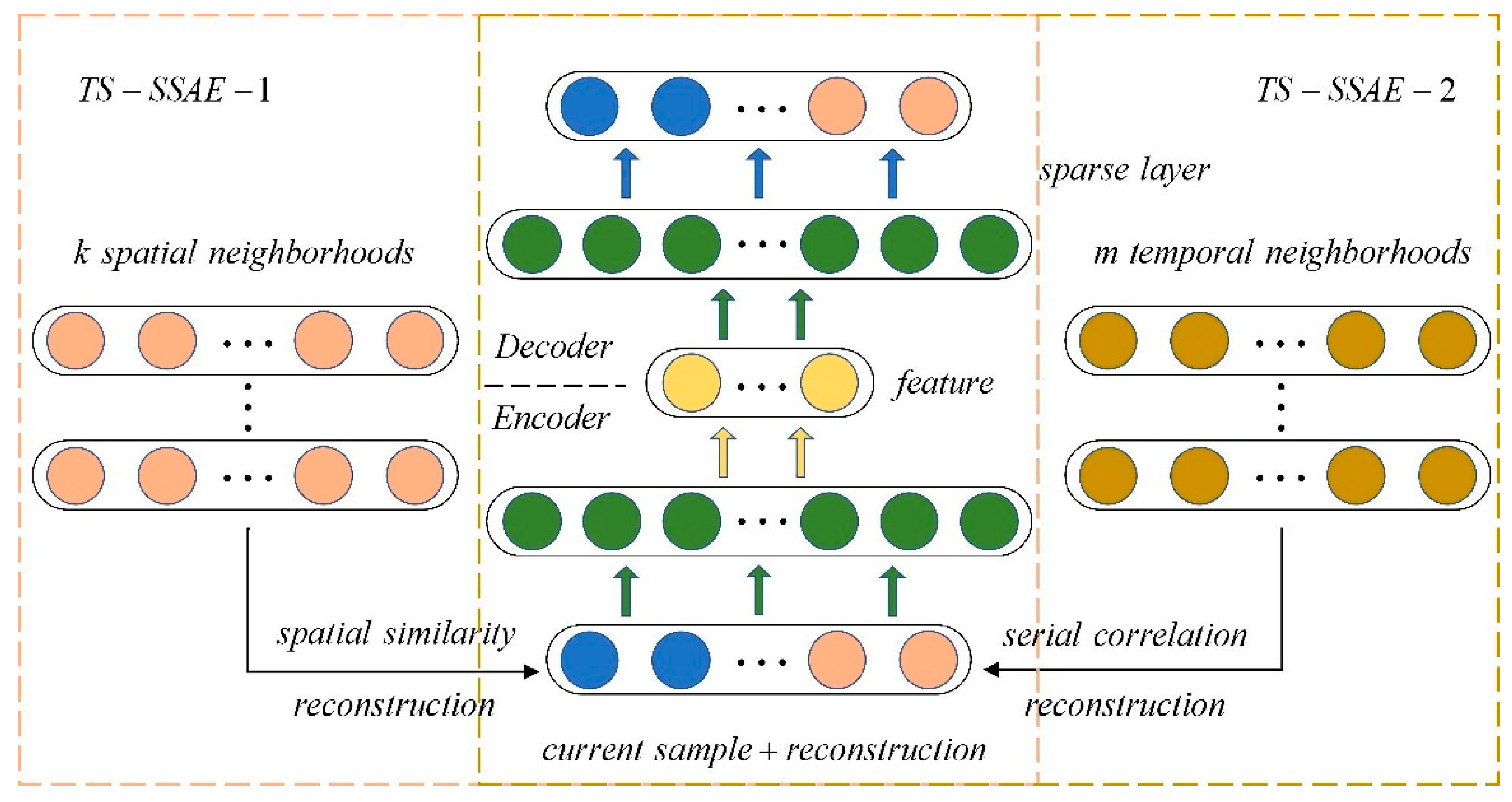
In the industrial process, for the current sample, there are spatial neighborhoods and temporal neighborhoods. Spatial neighborhoods refer to a number of samples with the minimum distance from the current sample in the sample feature space. The distance can generally be measured by Manhattan distance, Euclidean distance, etc. Temporal neighborhoods refer to the multiple samples whose sampling time is closest to the current time. The NPE or TNPE algorithm extracts features by keeping the linear reconstruction relationship of the spatial or temporal neighborhoods and the current sample unchanged to reduce the dimension. Therefore, extracting features by considering the relationship between the neighborhood and the current sample is an effective method for fault detection. Considering that there are complex dynamic nonlinear relationships in industrial processes, some algorithms, such as TNPE, are only suitable for linear processes by constructing projection matrices; most neural networks, such as NPNN, which consider neighborhoods, do not consider the time correlation. Therefore, TS-SSAE is proposed in this paper. For the spatial neighborhood selected within the time window, the timing constraint with the current sample is considered. For the temporal neighborhood, the spatial similarity with the current sample is also considered. Then, the neighborhood reconstruction information and the sample at the current time are combined as an input of SSAE to extract important information of the current sample and the neighborhood. The proposed algorithm can be divided into two parts according to the neighborhood object, which will be described in detail below.

Firstly, the original process data matrix is defined as $X=\left(x_1,x_2,\cdots ,x_n\right)\in R^{m\times n}$, where n is the number of samples, and m is the number of variables. Considering the dynamic characteristics of the process, the current sample can only use historical samples and samples of future moments cannot be obtained. Therefore, the time window L is defined as a time delay window, L = 2k is generally selected, and k is the number of spatial neighbors selected [23]. The TS-SSAE algorithm is composed of TS-SSAE-1 and TS-SSAE-2, and their neighborhood information is different. In TS-SSAE-1, for the current sample $x_t$, KNN is used to select k spatial neighbors from the time window L=$\left(x_{t-1},x_{t-2},\cdots ,x_{t-L}\right)$; they can be represented as $X_t^s=\left(x_{t-j_1},x_{t-j_2},\cdots ,x_{t-j_k}\right)$, and $x_{t-j_i}$ represents the ith spatial neighbor of the current sample $x_t$, $j_i$, which represents the time deviation from the current moment. There is a dynamic relationship between the sample in the appropriate time window and the current moment, and these neighbors have the smallest Euclidean distance from $x_t$, so they can be considered to have a high correlation with $x_t$ [24,25]. Since the construction of the neighborhood expansion matrix will increase the dimension of the variable, in this paper, we propose to reconstruct neighbors by time or space weight for using neighborhood information to assist in fault detection at the current time. The specific steps of TS-SSAE-1 are as follows:

(1) Calculate the time weight. For the spatial neighbors $X_t^s=\left(x_{t-j_1},x_{t-j_2},\cdots ,x_{t-j_k}\right)$, we consider the serial correlation in the time scale. First, the time distance between each neighbor and the current sample $x_t$ is calculated, and then the time weight can be constructed. The time distance can be defined as Equation (4), $T{D}_{ti}$ considers the degree of time deviation of all k spatial neighbors, and convert it to the serial correlation contribution of the ith neighbor to the current sample. What is more, the Gaussian kernel function is introduced to strengthen the time constraints at different times. Finally, the time weight is defined as Equation (5), and the weight of each neighbor is represented as $w_{t,i}$, the sum of the weights is set to be 1.

$$T{D}_{ti}=\frac{j_i}{{\displaystyle \sum _{i=1}^k{j}_i}}$$

(4)

$$w_{t,i}=e^{-T{D}_{ti}}/{\displaystyle \sum _{i=1}^k{e}^{-T{D}_{ti}}}$$

(5)

Based on the time weight $w_{t,i}$, the spatial neighbors can be reconstructed as Equation (6):

$$x_t^{r1}={\displaystyle \sum _{i=1}^k{w}_{t,i}{x}_{t-j_i}}$$

(6)

The reconstructed sample $x_t^{r1}$, obtained by Equation (6), means that the neighbors with high similarity are reconstructed by time serial correlation to expand the current sample as the neighborhood feature.

(2) Construct a TS-SSAE model. A TS-SSAE-1 model is based on the spatial neighbors, and the serial correlation is used as time weight to reconstruct neighbors for expanding the current sample $x_t$.Therefore, it also considers the topological structure of time and space. The input at the current time can be represented as $X_t^1=(x_t,x_t^{r1})$, and $X_t^1$ will be used as input for SSAE, the objective function is shown in Equation (7), and the sparsity restriction makes the extracted middle-layer features contain the most important information about the current sample and the reconstructed neighborhood.

$$J_{TS-SSAE}=\frac{1}{n}({\displaystyle \sum _{i=1}^n{\Vert {\stackrel{⌢}{x}}_i-x_i\Vert }_2^2}+\beta {\displaystyle \sum _{i=1}^n{\Vert h_j(W^{(j)}{z}_i)\Vert }_1})$$

(7)

The left part of Equation (7) is the reconstruction error of the autoencoder, and it should be noted that the sparsity parameter in the KL distance mentioned above is used as a hyperparameter, its choice has a greater impact on the result, and its value will be changed for a different dataset. Therefore, L1 regularization is applied to the hidden layer at each moment to avoid the design of hyperparameters. The objective function is the right part of Equation (7), $\beta$ is the weight that controls the sparsity penalty, $h_j$ is the output of the jth hidden layer, $z_i$ is the input of the jth hidden layer, and is also the output of the j-1th layer.

In TS-SSAE-1, the spatial neighborhood is the main body, but the temporal neighbors of $x_t$ have a more apparent serial correlation with $x_t$, the addition of temporal neighborhood information will be beneficial to deal with dynamic problems. In TS-SSAE-2, the temporal neighbor is used to reconstruct neighborhood information. First, for the current sample $x_t$, select m temporal neighbors in the time window L; they can be represented as $X_t^t=\left(x_{t-1},x_{t-2},\cdots ,x_{t-m}\right)$. The algorithm steps are as follows:

(1) Calculate spatial weights. For the temporal neighbors $X_t^t=\left(x_{t-1},x_{t-2},\cdots ,x_{t-m}\right)$ of the current sample $x_t$, we consider the similarity in the spatial scale. The spatial similarity is defined by Equation (8), and then the spatial weights are calculated according to Equation (9). The introduction of spatial similarity makes the reconstructed samples take into account the correlation between time and space at the same time. The defined reconstruction expression is shown in Equation (10):

$$D_{tj}=\frac{{\Vert x_t-x_{t-j}\Vert }_2^2}{{\displaystyle \sum _{j=1}^m{\Vert x_t-x_{t-j}\Vert }_2^2}},\hspace{1em}{x}_{t-j}\in X_t^t$$

(8)

$$w_{t,j}=e^{-D_{tj}}/{\displaystyle \sum _{j=1}^m{e}^{-D_{tj}}}$$

(9)

$$x_t^{r2}={\displaystyle \sum _{j=1}^m{w}_{t,j}{x}_{t-j}}$$

(10)

(2) Construct the TS-SSAE model. Similar to the TS-SSAE-1 section above, $X_t^2=(x_t,x_t^{r2})$ will be the input of SSAE, its objective function is the same as Equation (7), and the structure of TS-SSAE model is shown in Figure 2.

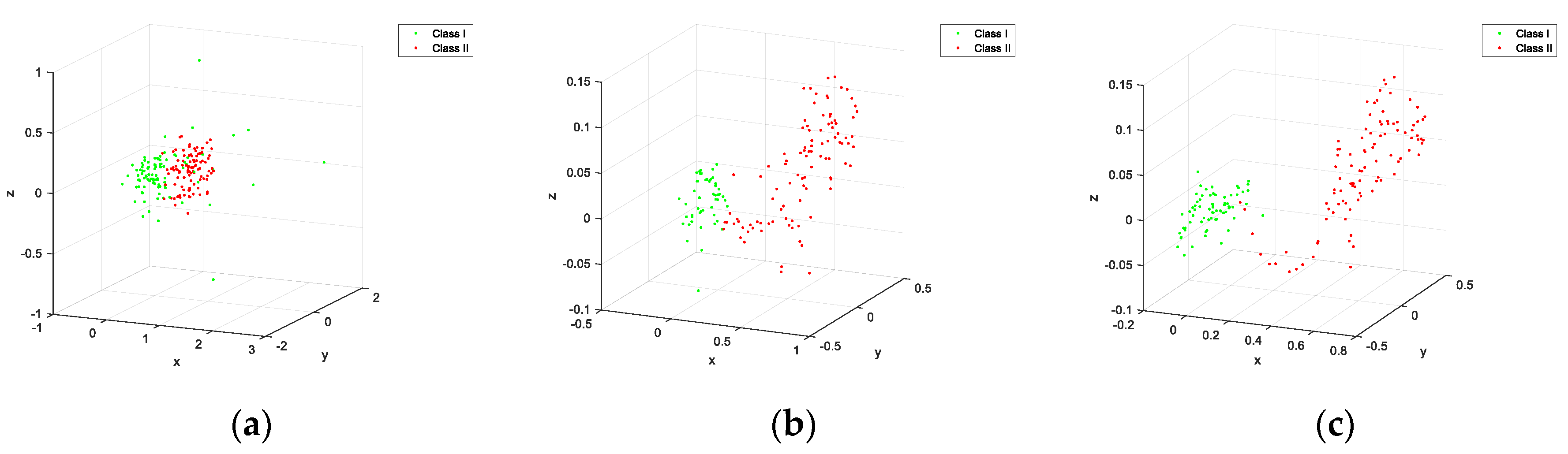
The TS-SSAE model considers the information of the distance in the time scale for spatial neighbors, and the spatial constraints for the temporal neighbors, both of which take into account spatial-temporal information, so they are suitable for feature extraction in dynamic processes. Besides, three points need to be explained here: (1) Neighbor reconstruction samples are used as input, which is equivalent to each neighbor being used as input at the same time, and each neighbor is given an importance coefficient and then shares the weight of the input layer. Therefore, the method of using neighborhood reconstruction as input can be considered to extract important information of each neighborhood in some way. (2) The two neighborhood weighted reconstructions mentioned above can improve the separability of sample points and achieve smooth denoising. So, it can be used as supplementary information of $x_t$ to reflect the different characteristics of each sample. The specific effect can be shown by the dataset constructed in Section 5. (3) For dynamic processes, dynamic data with similar sampling times have small changes, so the time neighborhood of the data may also be its spatial neighborhood. Obviously, for different dynamic processes, the overlap of the two neighborhoods is also different. However, the number of temporal neighborhoods and spatial neighborhoods selected in this paper are different. Even if the number of overlaps is large, since the weights of the two kinds of neighborhood reconstruction samples consider the time scale and the space scale, respectively, they will still provide different features.

4. Fault Detection Based on TS-SSAE

In this chapter, the TS-SSAE model proposed above is used for fault detection, the $T^2$ statistic is constructed by using the features of the middle layer, and the SPE statistic is also constructed by residual features. Finally, kernel density estimation (KDE) is used to establish control limits for fault detection. It is worth mentioning that the introduction of neighborhood reconstruction makes SSAE extract the correlation features between $x_t$ and neighbors, and reconstructed samples that integrate the characteristics of spatial and temporal neighbors provide richer information for $x_t$. When the fault occurs at the sampling time t, and the relationship between $x_t$ and the spatial-temporal neighbors changes, the obvious change of reconstructed samples will change the features extracted from the network for fault detection, which is also consistent with the separability mentioned above. Considering the temporal and spatial characteristics of the data in both parts of TS-SSAE, the Bayesian fusion strategy is used to integrate the two $T^2$ statistics and two SPE statistics to improve detection performance. We assume that the offline process dataset can be represented as $X=\left(x_1,x_2,\cdots ,x_n\right)\in R^{m\times n}$. According to the above algorithm, TS-SSAE-1 reconstructs the spatial neighbors to $x_t^{r1}$ and then makes $X_t^1=(x_t,x_t^{r1})$ the input of SSAE, the extracted middle layer feature is $h^1\left(x_i\right)\in R^{d1}$, and the reconstructed output is ${\stackrel{⌢}{X}}_t^1$. Similarly, TS-SSAE-2 takes the reconstructed temporal neighborhood $X_t^2=(x_t,x_t^{r2})$ as input, the feature of the middle layer is $h^2\left(x_i\right)\in R^{d2}$, and the reconstructed output is ${\stackrel{⌢}{X}}_t^2$, where d1 and d2 are the dimensions of the middle layer of the two networks. Considering that the calculation of the neighborhood requires samples in the time window L, for the online sample $x_{new}$, it is also necessary to set the time window and select the corresponding spatial-temporal neighborhood. Then, the pre-processed x1 and x2 are used as input into the two offline-trained SSAE models to obtain the feature representation $h^1\left(x_{new}\right)$ and $h^2\left(x_{new}\right)$, and the reconstructed feature ${\stackrel{⌢}{x}}_{new}^1$ and ${\stackrel{⌢}{x}}_{new}^2$. Then, the $T^2$ and $SPE$ statistics corresponding to $x_{new}$ can be constructed as Equations (11)–(13):

$$T_i^2=h^i{\left(x_{new}^i\right)}^T{\Lambda }_i^{-1}{h}^i\left(x_{new}^i\right)$$

(11)

$$SP{E}_i={\Vert x_{new}^i-{\stackrel{⌢}{x}}_{new}^i\Vert }^2$$

(12)

$${\Lambda }_i=\frac{1}{n-1}{\displaystyle \sum _{j=1}^n{h}^i\left(x_j\right)}{h}^i{\left(x_j\right)}^T$$

(13)

where i = 1,2, represents the detection results of TS-SSAE-1 and TS-SSAE-2, respectively, and Equation (13) represents the covariance of the feature layer of the offline training set.

The establishment of statistical control limit is an important factor to determine whether a fault occurs. There are two main ways to determine the control limit. One is to calculate the control limit by the empirical distribution under a certain confidence level, $\alpha$, when the feature variable obeys the Gaussian distribution [26,27]. The other is determined by kernel density estimation (KDE). KDE is a procedure for fitting a data set with a suitable smooth probability density function (PDF) from a set of random samples. It is used widely for estimating PDFs, especially for univariate random data [28]. The $T^2$ and SPE statistics are both univariate, although the process characterized by these statistics is multivariate. Therefore, KDE is widely used to establish control limits in recent studies [15,28,29]. In this paper, due to the complexity of the nonlinear transformation (for example, different activation functions have large differences), it is impossible to assume the feature layer distribution obtained by the neural network, that is, the feature distribution is unknown and does not necessarily obey the Gaussian distribution. Therefore, KDE is adopted in this paper to determine the control limits of $T^2$ and $SPE$ statistics, which can be denoted as $T_{\lim }^2$ [30].

In TS-SSAE, the spatial neighborhood reconstruction sample and the temporal neighborhood reconstruction sample represent different neighborhood information. Although the two types of neighborhoods may have a certain amount of overlap, the weight of the spatial neighborhood is based on the serial correlation, the weights of temporal neighborhoods take into account the spatial similarity, which means that their weights are determined according to different criteria. Moreover, the two parts of neighborhood reconstruction information consider the spatial and temporal neighborhood characteristics of $x_t$, so we choose to integrate the feature statistics $T^2$ and the residual statistics SPE extracted from the two parts of the network, respectively, in this paper, hoping to consider the influence of different neighborhoods more comprehensively. The integration method adopts the Bayesian fusion strategy. In this strategy, N and F represent normal conditions and fault conditions. The following takes $T^2$ as an example, integrates its detection results, and converts statistics into fault probability through Bayesian formulas [31,32,33]. The fault probability can be obtained by Equation (14).

$$P_{T_i^2}\left(F|x\right)=\frac{P_{T_i^2}\left(x|F\right)P_{T_i^2}\left(F\right)}{P_{T_i^2}\left(x\right)}$$

(14)

where i = 1,2, represents the monitoring results of the two networks, and $P_{T_i^2}\left(x\right)$ can be represented by Equation (15).

$$P_{T_i^2}\left(x\right)=P_{T_i^2}\left(x|N\right)P_{T_i^2}\left(N\right)+P_{T_i^2}\left(x|F\right)P_{T_i^2}\left(F\right)$$

(15)

In the above equation, $P_{T_i^2}\left(N\right)$ and $P_{T_i^2}\left(F\right)$ are, respectively, set as $1-\alpha$ and $\alpha$, where $\alpha$ is the confidence level. They are the prior probabilities of the process being normal and abnormal.

For a new sample, we can only obtain its conditional probabilities $P_{T_i^2}\left(x|N\right)$ and $P_{T_i^2}\left(x|F\right)$ according to its statistics. Moreover, what we expect is such a situation. Under normal conditions, the statistics of the samples will be less than the control limit, and the larger their deviation, the better, because this means a lower false alarm rate. That is, $P_{T_i^2}\left(x|N\right)$ has a higher probability below the control limit, and a smaller probability when it is higher than the control limit. Under abnormal conditions, the sample statistics will be higher than the control limit. Similarly, the larger the deviation, the better, which means that the algorithm has excellent fault detection capabilities. Furthermore, considering the uncertainty of the failure and the normalized property of the probability, we can assume that $P_{T_i^2}\left(x|F\right)$ has the following trend. When the statistic is lower than the control limit, there is a low probability, and when it is higher than the control limit, the probability is larger, and after reaching a certain peak, it starts to decrease slowly. Therefore, we define the conditional probability as Equations (16) and (17):

$$P_{T_i^2}\left(x|N\right)=\exp \left\{-\frac{T_i^2\left(x\right)}{v{T}_{i,\lim }^2}\right\}$$

(16)

$$P_{T_i^2}\left(x|F\right)\sim {\chi }^2\left(l\right),l>2$$

(17)

Equation (17) indicates that $P_{T_i^2}\left(x|F\right)$ with $\frac{T_i^2\left(x\right)}{v{T}_{i,\lim }^2}$ as the variable obeys the chi-square distribution of $l$ as the degree of freedom. $l$ and $v$ can be determined according to the actual situation. However, it is necessary to make the distribution of the two conditional probabilities intersect near the control limit, so that the probability of occurrence under normal conditions and the probability of occurrence under abnormal conditions can be balanced at the control limit. In this paper, we set $l$ as 5 and $v$ as 0.5.

Finally, the monitoring results of the new samples in the two parts of TS-SSAE, $T_1^2$ and $T_2^2$, $SP{E}_1$ and $SP{E}_2$ are gained, then the fault probability is weighted to obtain the final fused probabilistic statistics $BI{C}_{T^2}$ and $BI{C}_{SPE}$, as shown in Equation (18) [31,33]. The control limit of both is $\alpha$. Once the statistics of the Bayesian Inference Combination (BIC) exceed the control limit, the fault is considered to happen.

$$BI{C}_{T^2}={\displaystyle \sum _{i=1}^2\left\{\frac{P_{T_i^2}\left(x|F\right)P_{T_i^2}\left(F|x\right)}{{\displaystyle \sum _{i=1}^2{P}_{T_i^2}\left(x|F\right)}}\right\}}$$

(18)

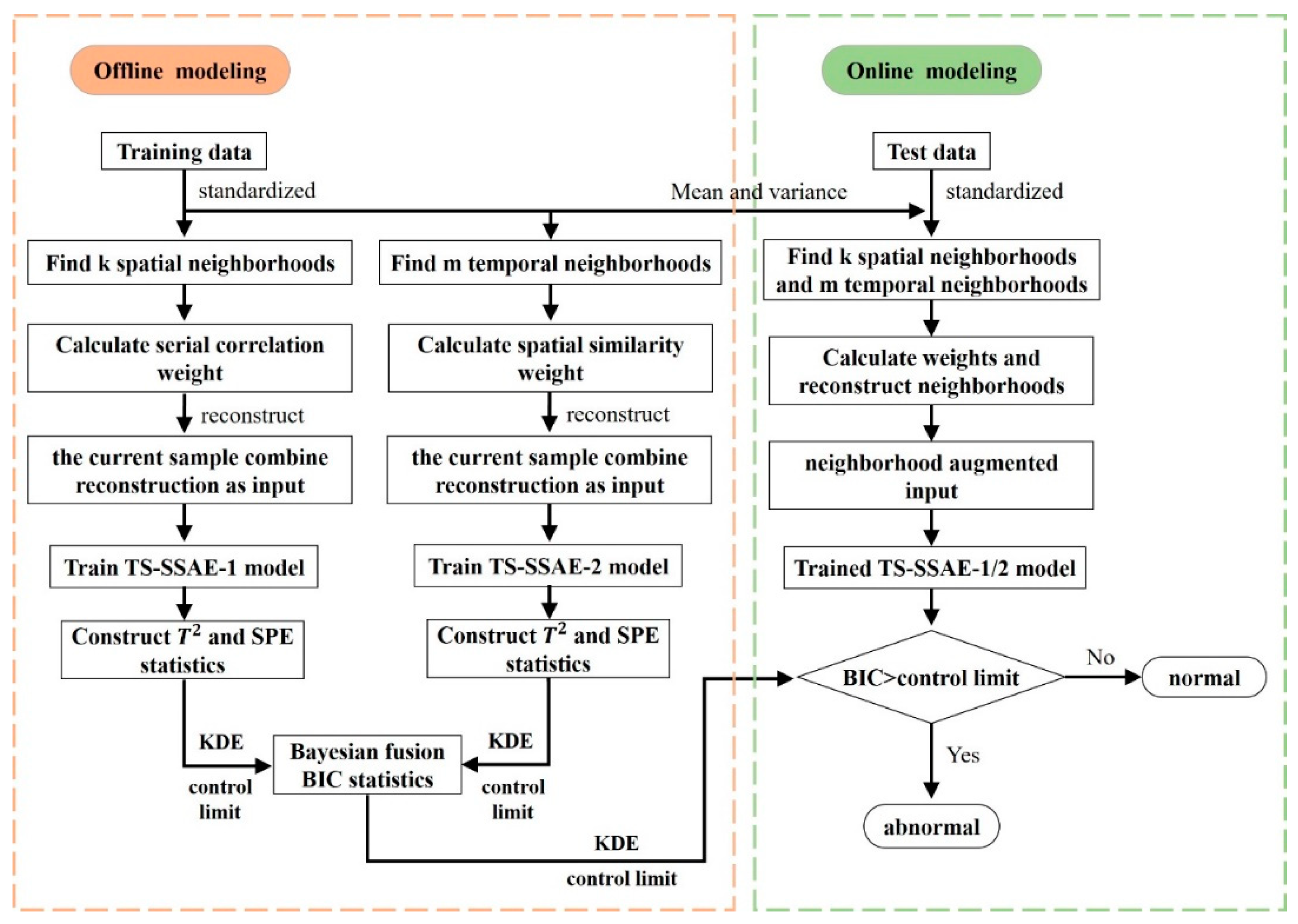
The steps of using the TS-SSAE algorithm for fault detection are summarized as follows. Figure 3 shows the flowchart of proposed method for fault detection.

4.1. Offline Modeling Steps

Step 1. The training sample data set $X\in R^{m\times n}$ is collected under normal conditions and standardizes it.

Step 2. Select the appropriate time window L and obtain the spatial neighborhood $X_t^s$ for each offline sample $x_t$ according to the KNN, and calculate the neighborhood reconstruction $x_t^{r1}$. Then, obtain the temporal neighborhood $X_t^t$ based on the serial correlation, and calculate the neighborhood reconstruction $x_t^{r2}$.

Step 3. Use the combined sample $X_t^1=(x_t,x_t^{r1})$ as input to train the SSAE model, which can be recorded as TS-SSAE-1, and obtain the feature of middle layer $h^1\left(x_t\right)$ and reconstructed output ${\stackrel{⌢}{X}}_t^1$. Similarly, the second SSAE is trained with the combined sample $X_t^2=(x_t,x_t^{r2})$ as input, which is denoted as TS-SSAE-2, and the features $h^2\left(x_t\right)$ and ${\stackrel{⌢}{X}}_t^2$ are obtained.

Step 4. Calculate their statistics $T^2$ and SPE respectively, and calculate their control limit by kernel density estimation (KDE). Finally, BIC is obtained by using Bayesian fusion strategy.

4.2. Online Monitoring Steps

Step 1. The test sample is standardized.

Step 2. Obtain the temporal and spatial neighbors within the time window L, and calculate the neighborhood reconstruction $x_{new}^{r1}$ and $x_{new}^{r2}$ according to Equation (2).

Step 3. $x_{new}^1=\left(x_{new},x_{new}^{r1}\right)$ and $x_{new}^2=\left(x_{new},x_{new}^{r2}\right)$ are input into the TS-SSAE-1 and TS-SSAE-2 trained in the offline step (3), respectively, and then the feature $h^1\left(x_{new}\right)$,$h^1\left(x_{new}\right)$ and the reconstructed feature ${\stackrel{⌢}{x}}_{new}^1$, ${\stackrel{⌢}{x}}_{new}^2$ can be obtained.

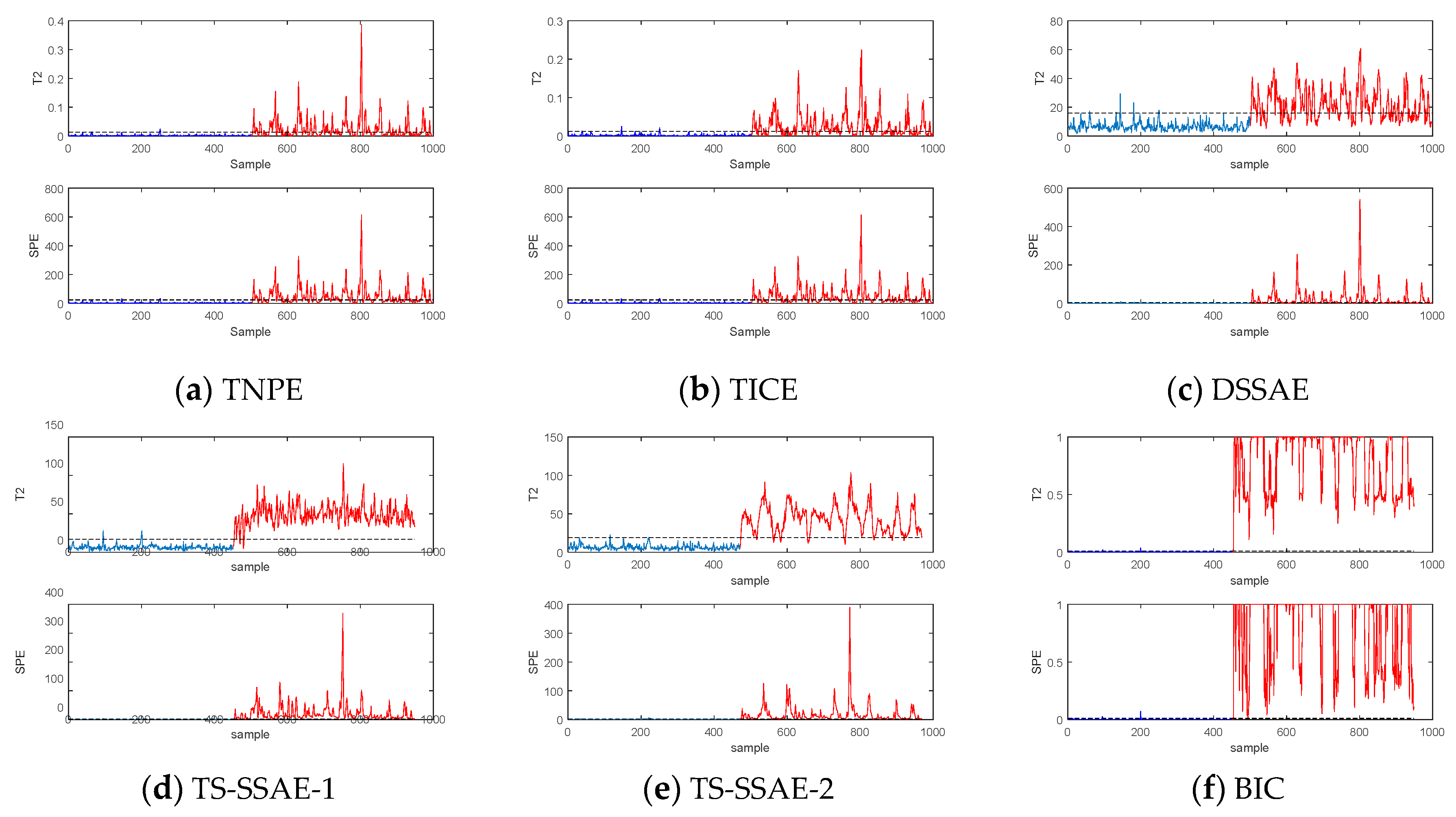
Step 4. According to Equations (11) and (12), two sets of $T^2$ and $SPE$ statistics are calculated, respectively, and the final fused probabilistic statistics $BI{C}_{T^2}$ and $BI{C}_{SPE}$ are also calculated. When $BIC>\alpha$, a fault is detected.

5. Case Study

In this paper, the proposed TS-SSAE algorithm is applied to the fault detection of a nonlinear dynamic process and the Tennessee-Eastman process to illustrate the effectiveness of the proposed algorithm. Considering the industrial dynamic process in this paper, the time information constrained embedding algorithm (TICE) also considers the spatial neighborhood and its serial correlation in the time window [30]. The TNPE algorithm has been widely used in fault detection as a method to deal with the serial correlation of data. Besides, the DSSAE algorithm based on the augmented matrix also extracts the dynamic nonlinear features of data. Therefore, we compare the proposed fault detection algorithm based on TS-SSAE with the above algorithm to indicate its superiority in this chapter.

5.1. Neighborhood Reconstruction

In this section, a model with the dynamic correlation that follows Equation (19) is adopted to construct the data set, including two types of data. Class I can be considered as normal samples, and class II data as samples under abnormal conditions.

$$\{\begin{array}{l}x\left(t\right)=A_{1}x\left(t-1\right)-A_{2}x\left(t-2\right)+e\left(t\right)\\ y\left(t\right)=P_{1}x\left(t\right)+v\left(t\right)\end{array}$$

(19)

$$\begin{gathered} A_1=\left[\begin{array}{ccc}0.4389& 0.1210& -0.0862\\ -0.2966& -0.0550& 0.2274\\ 0.4538& -0.6573& 0.4239\end{array}\right],A_2=\left[\begin{array}{ccc}-0.2998& -0.1905& -0.2669\\ -0.0204& -0.1585& -0.2950\\ -0.1461& -0.0755& 0.3749\end{array}\right], \\ {P}_1=\left[\begin{array}{ccc}0.5586& 0.2042& 0.6370\\ 0.2007& 0.0492& 0.4429\\ 0.0874& 0.6062& 0.0664\end{array}\right] \end{gathered}$$

where $e$,$v\sim N\left(0,{0.1}^2\right)$, step change occurs at t = 101 to construct two kinds of data to study the reconstruction effect, that is, $x\left(101\right)=A_{1}x\left(100\right)-A_{2}x\left(99\right)+e\left(101\right)+{\left[0.1,-0.1,0\right]}^T$. Figure 4 shows the results after neighborhood weighted reconstruction.

It can be found from the data distribution of Figure 4b,c that, compared with the original data distribution, the spatial neighborhood reconstruction with serial correlation and the temporal neighborhood reconstruction with spatial similarity can indeed make the difference between different types of data obvious. This means that it is more separable, and some of the noise points in Figure 4a are removed. It has been emphasized in Section 2 above that such a property will cause abnormal changes in the reconstructed samples of different neighborhoods when the fault occurs, so that the relationship between the reconstructed samples, and the current sample $x_t$ will change and the extracted feature statistics will be abnormal.

5.2. Numerical Case

A typical nonlinear dynamic system is used to verify the fault detection based on TS-SSAE proposed in this paper, and compares it with TNPE, TICE and other basic algorithms. The given data model is as Equation (20).

$$\{\begin{array}{l}{u}_0\left(t\right)=G{u}_0\left(t-1\right)+Hw\\ x\left(t+1\right)=Ex\left(t\right)+Ff\left(u_0\left(t\right)\right)\\ y\left(t\right)=x\left(t\right)+v\\ u\left(t\right)=u_0\left(t\right)+z\end{array}$$

(20)

In this model, $u\in R^2$, $y\in R^2$, and $x\in R^2$ are the input, output, and state variables of the dynamic system, respectively. f is a nonlinear mapping function: $f\left(u\right)={\left[{\left(u^1\right)}^2,{\left(u^2\right)}^2\right]}^T$, and then u and y are used as monitoring variables for fault detection. Where the measured noise v and z of the input and output variables are random noises that generated by $N\left(0,0.1\right)$, the process noise of the input variable is generated by $N\left(0,1\right)$. The dynamic relationship of the system is controlled by four matrices: E, F, G and H.

$$E=\left[\begin{array}{cc}0.118& -0.191\\ 0.847& 0.264\end{array}\right],F=\left[\begin{array}{cc}0.05& 0.1\\ 0.05& 0.05\end{array}\right],G=\left[\begin{array}{cc}0.811& -0.226\\ 0.477& 0.415\end{array}\right],H=\left[\begin{array}{cc}0.193& 0.689\\ -0.320& -0.749\end{array}\right]$$

Under normal conditions, 1000 normal pieces of data are collected as a training set. After that, another 1000 pieces of data will be collected as the test sample set, in which the test samples introduce the following two kinds of faults at the 501st data point:

Fault 1: the first-dimensional variable of input $u_0\left(t\right)$ produces a step change of magnitude 1.

Fault 2: 0.1 in row 1 and column 2 of coefficient matrix F changes to -1 (that is, the dynamic relationship of variable changes).

The offline training set is used to reconstruct two parts of the neighborhood within the time window, then the TS-SSAE-1 and TS-SSAE-2 models are trained for fault detection. The structure of the network is 8-20-5-20-8, which can be determined according to the reconstruction error, and the objective function is selected as Equation (7). We set two sparse layers with 20 units, the hyperparameter $\beta$, time window L, spatial neighborhood number k, and temporal neighborhood number m are set to ${10}^{-4}$, 50, 25, and 10, respectively. For the two designed faults, the $T^2$ and $SPE$ statistics are considered and then the fused probabilistic statistic BIC is established. We evaluate the detection effect by missing alarm rate (MAR) and false alarm rate (FAR). The missing alarm rate and false alarm rate can be defined in Equations (21) and (22), positives represent normal samples, and negatives represent fault samples [26].

$$MAR=\frac{falsenegatives}{totalnumberofnegatives}$$

(21)

$$FAR=\frac{falsepositives}{totalnumberofpositives}$$

(22)

According to the FAR in

Table 1. Result of fault detection in the case study (FAR) /%.

TNPE		TICE		DSSAE		TS-SSAE-1		TS-SSAE-2		BIC
$T^2$	SPE	$T^2$	SPE	$T^2$	SPE	$T^2$	SPE	$T^2$	SPE	$T^2$	SPE
0.80	0.80	1.40	0.80	1.40	1.40	0.56	0.78	0.64	1.16	0.77	1.33

, it can be found that the FAR of the four methods are similar, and they are all kept at a low value, which can ensure the effectiveness of the alarm. On the other hand, the lower miss alarm rate represents a better detection effect.

Table 2. Result of fault detection in the case study (missing alarm rate (MAR)) /%.

Fault	TNPE		TICE		DSSAE		TS-SSAE-1		TS-SSAE-2		BIC
	$T^2$	$SPE$	$T^2$	$SPE$	$T^2$	$SPE$	$T^2$	$SPE$	$T^2$	$SPE$	$T^2$	$SPE$
1	52.20	42.80	41.20	42.20	34.87	35.07	1.60	2.41	6.41	4.20	0.60	0.60
2	48.80	37.80	43.40	37.40	19.64	16.43	8.42	1.60	1.20	0.40	1.00	0.40

shows the MAR of the four algorithms, in which the network structure parameters of the DSSAE model are the same as those of the TS-SSAE model. It can be seen that the detection algorithm based on TS-SSAE has a significantly lower MAR than the other three methods, which means its detection effect is relatively better. Considering that fault 1 is a nonlinear fault, TNPE and TICE extract features by using a linear transformation of the projection matrix, so the detection effect is relatively poor, and the DSSAE model extracts dynamic nonlinear features by constructing an augmented matrix with time delay and its detection effect is indeed better than that of linear methods such as TNPE. However, compared with the BIC results of the TS-SSAE algorithm, there is still a large gap, which also reflects the excellent detection ability of the TS-SSAE detection method for nonlinear faults. Fault 2 is the change of the dynamic relationship of variables. It can be found from the table that, for this type of fault in nonlinear processes, the detection effect of traditional methods such as TNPE and TICE is not ideal, and the MAR is high. The detection ability of the DSSAE algorithm has been significantly improved, but, compared with the TS-SSAE method, the detection method based on the TS-SSAE still maintains the optimal detection effect, and the MAR is obviously lower. This shows that TS-SSAE also has great advantages in dealing with the dynamic characteristics of data. The method based on neighborhood reconstruction will provide more effective dynamic correlations than the delay augmented matrix. What is more, the fused probabilistic statistics BIC of the two parts of TS-SSAE further integrates the detection results of two kinds of neighborhood information, which further improves the detection effect. Figure 5 and Figure 6 show the detection results and control limits of the four methods, and the TS-SSAE method includes TS-SSAE-1, TS-SSAE-2 and the integrated indicator BIC, which all contain $T^2$ and SPE statistics.

5.3. Tennessee Eastman Process

The Tennessee-Eastman process (TE process) provides a practical industrial process simulation platform for the assessment of process control strategies and process monitoring algorithms, mainly including five units: reactor, condenser, compressor, separator and stripper [34]. The entire process includes 53 variables, including 12 manipulated variables, 22 continuous process variables, and 19 composition measurement variables. The agitator speed is considered to remain unchanged and is generally not considered. In order to evaluate the performance of various monitoring algorithms, 21 faults are set previously for the purpose of process monitoring. In this experiment, a total of 33 variables including 11 control variables and 22 process measurement variables are selected as the monitored variables. Under normal conditions, 960 samples are collected as the offline training set, and the testing set collects 960 samples after adding the fault from the 161st sample [35,36,37].

The structure of TS-SSAE model is set as 66-120-48-120-66, which can be selected according to the reconstruction error, and the hyperparameter, time window L, spatial neighborhood number k, temporal neighborhood number m are set as 50, 25, 10, respectively [38]. For comparative experiments, considering that the sample most relevant to the ith sample in TE process is the i-1th sample, the delay of the DSSAE model is set as 1, and the same structure as the TS-SSAE model is adopted. The temporal neighborhood number m in TNPE is 25, and the spatial neighborhood number K in TICE is 38. Under this condition, the performance of the algorithm is kept at an optimal level, which is more conducive to evaluating the performance of the proposed algorithm.

In order to demonstrate the effectiveness of TS-SSAE’s fault detection scheme, false alarm rate (FAR) and missing alarm rate (MAR) are introduced as evaluation indexes. False alarm rate can be defined as the probability of false alarm in the normal sample set [39]. The FAR of the four methods in the normal data set during TE simulation is shown in

Table 3. Monitoring results of normal data in the Tennessee-Eastman process (FAR) /%.

TNPE		TICE		DSSAE		TS-SSAE-1		TS-SSAE-2		BIC
$T^2$	SPE	$T^2$	SPE	$T^2$	SPE	$T^2$	SPE	$T^2$	SPE	$T^2$	SPE
2.60	1.40	2.20	1.40	1.60	5.01	0.89	3.34	2.44	3.46	0.89	2.89

. It can be seen that the FAR of the four methods is kept at a low level, which can ensure the effectiveness of monitoring. Although the FAR of the monitoring scheme based on TS-SSAE is slightly higher than that of TNPE and other methods, considering that its value is still in a reasonable scope, the decrease in the MAR indicates that its ability to detect faulty samples will be greatly improved, so the scheme still has a higher advantage under the balance.

Table 4. Results of 21 faults detection in the Tennessee-Eastman process (MAR) /%.

Fault	TNPE		TICE		DSSAE		TS-SSAE-1		TS-SSAE-2		BIC
	$T^2$	SPE	$T^2$	SPE	$T^2$	SPE	$T^2$	SPE	$T^2$	SPE	$T^2$	SPE
1	0.50	0.75	0.13	0.75	0.13	0,13	0.25	0	0.13	0.13	0.13	0
2	2.38	1.75	2.50	1.75	1.75	1.63	2.13	1.13	1.38	1.75	1.38	1.38
3	98.63	99.25	97	99.25	97.63	93.75	84.38	86	87.63	90.88	87.13	86.75
4	2.13	41	0	41	0	0	0.13	0	0	0	0	0
5	0	77	0	75.25	0	0	0.13	0	0	0	0	0
6	0	0	0	0	0	0	0	0	0	0	0	0
7	0.75	0	0.13	0	0	0	0	0	0	0	0	0
8	3.50	2.50	3.88	2.50	2	1.88	1.88	1.25	1	1	1.13	1
9	98.38	99	97.63	99	96	94.88	94.13	91.88	86.88	91.63	91.12	90.75
10	14.25	61.13	11.88	61.13	13.88	24	5	8.38	3.38	10.75	3	6.38
11	34.50	45.50	32.50	45.50	12.13	6.75	11.13	4.25	5.13	2.75	4.50	1.63
12	0.38	1.63	0.25	1.63	0.38	0.50	0.25	0.25	0.13	0.25	0.13	0.25
13	5	5.75	4.88	5.75	4.63	4	4.63	4.38	3.88	4.25	4.13	4.25
14	0	0.13	0.13	0.13	0	0	0	0	0.13	0	0	0
15	96.63	97	94.13	97	96.50	92.50	93.50	83.13	85.88	88.38	89.38	84.12
16	11.75	79.25	9.38	79.50	8.75	28.50	1.50	3.50	2.25	9.13	0.88	1.88
17	5.75	14.13	7.63	14.13	3.75	1.88	2.50	2	2.25	2.38	2.25	2.13
18	10.13	10.75	9.88	10.75	9.75	9.38	10.25	9.13	9.38	9.13	9.63	9.25
19	21	98.13	13.75	98.13	3.50	16.25	8.25	11.50	3	18.25	0.88	8.12
20	9.63	58.38	11.63	58.38	23.50	27.63	7.50	8	9.38	8.75	8.5	8.12
21	63.63	61.75	56.63	61.75	50.75	49.75	35.38	28.75	41.13	29.13	33.25	27.12

shows the MAR of the four algorithms under the 21 faults in the TE process. According to the definition of the MAR, the smaller the value, the better the detection effect of the algorithm. By comparing the minimum MAR of four algorithms for each fault, the detection effect of each algorithm is evaluated. It can be found from the comparison in Table 4 that the fault detection scheme based on the TS-SSAE model has a better detection effect for the 18 types of faults other than faults 3, 9, and 15, because these three types of faults have only a small fluctuation compared to the normal state, which is more difficult to detect for most algorithms, but the MAR of the TS-SSAE algorithm is still lower than that of the other three algorithms. It is worth noting that the detection scheme based on TS-SSAE proposed in this paper finally determines whether the fault occurs according to the BIC index, and the strategy of integrating the feature layer and residual layer of two networks separately will improve the detection effect of some faults by comparing the MAR of TS-SSAE-1, TS-SSAE-2 and BIC, such as fault 10,16, etc. For some faults that have not been improved, the MAR will also be kept near the optimal effect. Therefore, BIC will be used as the only index of TS-SSAE detection scheme in the following experimental comparison. Among the other 18 kinds of faults, for faults 5, 10, 16, 19 and 20, which are difficult to detect, the detection algorithm based on TS-SSAE has a significant advantage over the other three algorithms, and the MAR has decreased significantly. For faults that are easy to be detected, such as fault 4, 8, 12, 17, and so on, the four algorithms all have a good detection effect, but the overall TS-SSAE algorithm is still better. Even if the DSSAE algorithm has the best detection effect on fault 17, the difference is tiny. In addition, for fault 6, 7, and 14, all algorithms can almost achieve the complete detection effect, and, for fault 1, 2, 13, 18, the TS-SSAE algorithm has similar detection results with TNPE and other algorithms. It is worth mentioning that, for fault 21, the detection result based on the TS-SSAE algorithm is significantly better than the other three algorithms. Therefore, the following conclusions can be drawn from the comparison of MAR of 21 faults in Table 4: The fault detection effect of the TS-SSAE algorithm is generally superior to the TNPE and TICE algorithms, indicating that the fault detection scheme based on the TS-SSAE algorithm is more advantageous for dealing with dynamic process monitoring. Compared with the DSSAE algorithm, the detection effect of fault 13 and 17 is only slightly inferior but almost equal. In general, the TS-SSAE algorithm still has great advantages, which proves that the TS-SSAE algorithm can extract more effective nonlinear features with the help of neighborhood information and enhance the sensitivity of fault detection.

In order to describe the fault detection effect of different algorithms clearly, the following will give a detailed description of several types of faults and give specific detection results. First, we take fault 5 as an example, and the detection results of the four algorithms are shown in Figure 7. Fault 5 is a step change of the inlet temperature of cooling water of the condenser [40,41]. It can be found that the $T^2$ statistics of the four algorithms can quickly exceed the control limit when the fault occurs and remain above the control limit during the existence of the fault, so as to give an effective alarm. However, after this fault occurs, the output flow rate from the condenser to the separator increases, which causes the temperature in the separator and the outlet temperature of the cooling water to increase. Although most of the variables will resume to the steady-state value after adjustment by the controller, the inlet temperature and flow rate of the condenser cooling water are still abnormal, that is, the fault still exists [42]. The SPE statistics of the TNPE and TICE algorithm can still alarm immediately when the fault occurs, but the statistics will return to the normal state after the loop compensation, which will have an adverse impact on the fault detection. The $T^2$ and SPE statistics of the TS-SSAE and DSSAE algorithms will immediately exceed the control limit after the fault occurs, and maintain the fault alarm after the loop adjustment, indicating that the fault still exists. This shows that the SSAE will extract more effective residual features, and the features extracted by the TS-SSAE algorithm combined with the neighborhood information can provide fast and stable detection results.

Figure 8 shows the detection results of fault 10 with four algorithms. The four algorithms start to find faults at about 25 sampling points after the fault occurs. Among them, the $T^2$ statistics of each algorithm can be continuously alarmed after the fault is found, but it is evident that the TS-SSAE algorithm has a stronger ability to continuously alarm, which can be found from the result that the MAR of the $T^2$ statistics of BIC is better than other algorithms. In addition, comparing the SPE statistics of the three algorithms about fault 10 from Table 3 and Figure 8, it can be clearly found that the MAR of the SPE statistics of the TNPE, TICE and DSSAE algorithms is exceptionally high, and after the fault occurs, the continuous alarm cannot be performed, while the SPE statistics of the TS-SSAE algorithm has distinct advantages in comparison, so it can still perform effective continuous alarms. In summary, the comparison of the detection performance of the four algorithms shows that the proposed TS-SSAE algorithm still has excellent advantages in fault detection capability.

By the detection results of the TE process, it can be found that TICE is slightly better than the TNPE algorithm in overall detection, indicating that the idea of considering time constraints in the spatial neighborhood is conducive to the algorithm to extract more effective features. The conclusion that the detection effect of the TNPE algorithm is significantly better than that of the NPE and PCA algorithms also indicates that considering the dynamic correlations between data is an essential factor in improving the performance of process monitoring [7]. Compared with the above four algorithms, TS-SSAE shows the optimal detection capability in TE process, and the comparison with DSSAE algorithm shows that it has more advantages by using neighborhood information to combine the current samples for dealing with industrial process dynamic problems. Compared with the algorithm that only preserves the time or space structure, it can extract more effective features. Meanwhile, the nonlinear features extracted by SSAE will more effectively deal with the sophisticated nonlinear features in the industrial process, so as to provide a more accurate monitoring model.

6. Conclusions

In this paper, a spatial-temporal neighborhood enhanced sparse stack autoencoder is proposed. By weighted reconstruction of the spatial (temporal) neighborhood within the time window, the neighborhood supplementary information of the current sample is formed, and then the combined sample is used as input of SSAE to extract the practical features for fault detection. Considering that both kinds of neighborhood reconstruction information contain temporal and spatial characteristics, it is proposed to integrate the two parts of feature statistics based on Bayesian theory to improve the detection ability further. Finally, it is further demonstrated by a numerical case and TE process. By comparing with TICE and other algorithms, the detection scheme based on the TS-SSAE algorithm has certain advantages in dealing with nonlinear dynamic problems in industrial processes.

For the superiority of the TS-SSAE algorithm, we can make the following analysis: Firstly, the introduction of neighborhood reconstruction information makes the features extracted by the network contain the important information of current samples and neighborhoods, and the limitation of sparse layer further makes the features more representative. On the other hand, neighborhood reconstruction achieves smooth denoising and improves the separability of different types of data. It makes the reconstructed samples significantly change when the fault occurs; then, the characteristic statistics will be abnormal. Richer sample information makes the detection effect of the TS-SSAE algorithm better than that of the DSSAE algorithm because the DSSAE algorithm relies on the delay extension matrix, and more extensive delay means higher dimension. The extraction of nonlinear features makes the TS-SSAE algorithm significantly better than the TNPE algorithm because they only consider the linear relationship between the current sample and the neighborhood. Secondly, the introduction of Bayesian fusion strategy makes the algorithm comprehensively consider the temporal and spatial characteristics of the two neighborhoods, then the detection results of the two parts of the network are integrated. In general, the fault detection based on the TS-SSAE algorithm is effective. However, there are also some shortcomings. The selection and reconstruction of the neighborhood of each sample increase the complexity of the algorithm, which will affect the real-time performance of the detection during online monitoring. This is also one of the directions that need to be improved in the future.